Sentinel-2 L1C MSI Zarr Product Exploration

Table of Contents¶

Introduction
Import modules
Open the product
Overview of the product content
Plot a RGB image
Explore product geolocation
A. Interactive map
B. Non-interactive map
Compute radiances
Visualization

Run this notebook interactively with all dependencies pre-installed

Introduction¶

This notebook demonstrates how to open, explore, and visualize Sentinel-2 Level 1C MSI products stored in EOPF Zarr format, including plotting RGB images and analyzing geolocation data.

Import modules¶

import cartopy.crs as ccrs
import numpy as np
import matplotlib.pyplot as plt
import xarray as xr

ERROR 1: PROJ: proj_create_from_database: Open of /home/mclaus@eurac.edu/micromamba/envs/eopf-zarr3/share/proj failed

Open the product¶

remote_product_path = "https://objects.eodc.eu/e05ab01a9d56408d82ac32d69a5aae2a:sample-data/tutorial_data/cpm_v253/S2B_MSIL1C_20250113T103309_N0511_R108_T32TLQ_20250113T122458.zarr"
dt = xr.open_datatree(remote_product_path, engine="zarr", chunks={})

/home/mclaus@eurac.edu/micromamba/envs/eopf-zarr3/lib/python3.11/site-packages/xarray_sentinel/esa_safe.py:7: UserWarning: pkg_resources is deprecated as an API. See https://setuptools.pypa.io/en/latest/pkg_resources.html. The pkg_resources package is slated for removal as early as 2025-11-30. Refrain from using this package or pin to Setuptools<81.
  import pkg_resources
/tmp/ipykernel_3440119/938497852.py:2: FutureWarning: In a future version, xarray will not decode the variable 'step' into a timedelta64 dtype based on the presence of a timedelta-like 'units' attribute by default. Instead it will rely on the presence of a timedelta64 'dtype' attribute, which is now xarray's default way of encoding timedelta64 values.
To continue decoding into a timedelta64 dtype, either set `decode_timedelta=True` when opening this dataset, or add the attribute `dtype='timedelta64[ns]'` to this variable on disk.
To opt-in to future behavior, set `decode_timedelta=False`.
  dt = xr.open_datatree(remote_product_path, engine="zarr", chunks={})
/tmp/ipykernel_3440119/938497852.py:2: FutureWarning: In a future version, xarray will not decode the variable 'step' into a timedelta64 dtype based on the presence of a timedelta-like 'units' attribute by default. Instead it will rely on the presence of a timedelta64 'dtype' attribute, which is now xarray's default way of encoding timedelta64 values.
To continue decoding into a timedelta64 dtype, either set `decode_timedelta=True` when opening this dataset, or add the attribute `dtype='timedelta64[ns]'` to this variable on disk.
To opt-in to future behavior, set `decode_timedelta=False`.
  dt = xr.open_datatree(remote_product_path, engine="zarr", chunks={})

Overview of the product content¶

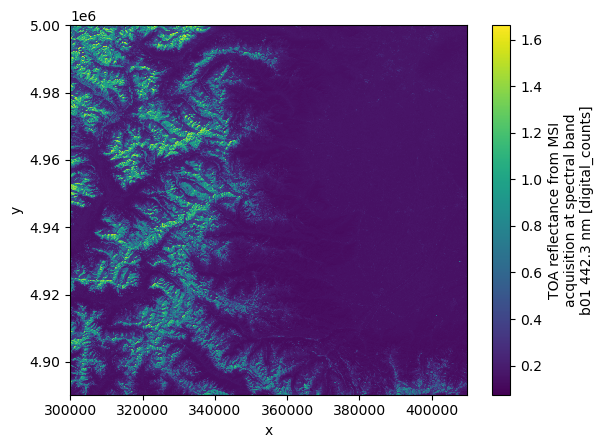
dt["measurements/reflectance/r60m"]["b01"].plot()
# Alternative notation
# dt.measurements.reflectance.r60m.b01.plot()

The original data is stored in uint16, with scale and offset values to be applied manually.
Xarray applies the scale and offset automatically, providing reflectance values by default.
You can still get the original Digital Numbers (DNs) in uint16 by setting the mask_and_scale = False parameter when opening the product, e.g.:

dt = xr.open_datatree(remote_product_path, engine="zarr", chunks={}, mask_and_scale=False)

We can get some info about the oroginal encoding with the following code:

dt["measurements/reflectance/r60m"]["b01"].encoding

{'chunks': (305, 305),
 'preferred_chunks': {'y': 305, 'x': 305},
 'compressor': Blosc(cname='zstd', clevel=3, shuffle=BITSHUFFLE, blocksize=0),
 'filters': None,
 '_FillValue': 0,
 'scale_factor': 0.0001,
 'add_offset': -0.1,
 'dtype': dtype('uint16')}

If we are interested in some band statistics, they can easily be computed using the xarray methods.
Remember that calling .compute() triggers the data download and processing of the result.

min, max, mean = (
    dt["measurements/reflectance/r60m"]["b01"].data.max(),
    dt["measurements/reflectance/r60m"]["b01"].data.min(),
    dt["measurements/reflectance/r60m"]["b01"].data.mean(),
)
min.compute(), max.compute(), mean.compute()

(1.6631, 0.0746, 0.27504428200304576)

Plot a RGB image¶

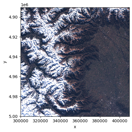
We can compose a new object for visualization, taking only the red (b04), green (b03) and blue (b02) bands.

Decimation is also applied, which reduces the data we consider for visualization, speeding up the process. Decimation is performed using the .isel xarray method.

.isel(x=slice(None, None, 10), y=slice(None, None, 10))

Finally, we rescale the data for a more meaningful visualization.

rgb_band_paths = (
    "measurements/reflectance/r10m/b04",
    "measurements/reflectance/r10m/b03",
    "measurements/reflectance/r10m/b02",
)
# Concatenate the selected bands in a single xarray DataArray, applying decimation with a factor of 10
concat = xr.concat(
    [
        dt[str(p)].isel(x=slice(None, None, 10), y=slice(None, None, 10))
        for p in rgb_band_paths
    ],
    dim="band",
)

# Rescale the data for a more meaningful visualization
concat = (concat / 0.4).clip(0, 1)

ax = concat.plot.imshow()
ax.axes.set_aspect("equal")
plt.gca().invert_yaxis()

Explore product geolocation¶

The Zarr product metadata contains information about the product geolocation we can explore in various ways.

Interactive map¶

The following code snippet shows an interactive map with the tile’s footprint

import geopandas as gpd

# Create a GeoDataFrame from the feature
gdf = gpd.GeoDataFrame.from_features(
    [
        {
            "type": "Feature",
            "geometry": dt.attrs["stac_discovery"][
                "geometry"
            ],  # Use the actual geometry, not the bbox
            "properties": dt.attrs["stac_discovery"][
                "properties"
            ],  # Include all properties
        }
    ],
    crs="EPSG:4326",  # Set the CRS explicitly (adjust EPSG code if needed)
)

gdf.explore()

Non-interactive map¶

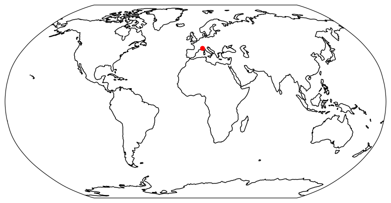
The following code snippet shows the location of the tile on a global map.

# Reproject to a projected CRS
gdf_projected = gdf.to_crs(epsg=3857)
centroids = gdf_projected.centroid

fig = plt.figure(figsize=(10, 5))
ax = fig.add_subplot(1, 1, 1, projection=ccrs.Robinson())

# Make the map global rather than have it zoom in to the extents of any plotted data
ax.set_global()

# ax.stock_img()
ax.coastlines()

# Transform back to geographic CRS for plotting
gdf_centroids_geographic = centroids.to_crs(epsg=4326)

ax.plot(
    gdf_centroids_geographic.x,
    gdf_centroids_geographic.y,
    "ro",
    transform=ccrs.PlateCarree(),
)

plt.show()

Compute radiances¶

From: https://s2.pages.eopf.copernicus.eu/pdfs-adfs/MSI/L1/PDFS_S2_MSI_L1C.myst.html#product-overview

$\text{radiance} = \text{reflectance} \times \cos\left(\text{radians}(\text{SunZenithAngle})\right) \times \text{solarIrradiance} \times \frac{U}{\pi}$ $ ]

U: float = dt.attrs["other_metadata"][
    "reflectance_correction_factor_from_the_Sun-Earth_distance_variation_computed_using_the_acquisition_date"
]
U

1.03411047670495

Be carefull, Sun Zenith Angle is expressed on the angles grid (5km), it needs to be reprojected on the 10m grid for computing radiances cosinus is applied now because we can not interpolate angles using a linear interpolation (discontinuity at 0°).
On the other hand, cosines can be interpolated:

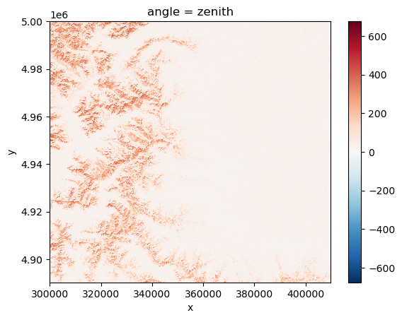
cos_sza_5km = np.cos(np.deg2rad(dt["conditions/geometry/sun_angles"])).sel(
    angle="zenith"
)
cos_sza_5km

# We will convert reflectances from band b02 to radiances
BAND: int = 2  # b02

# Band - 1 because Python list index starts at 0
solarIrradiance: float = np.float64(
    dt.attrs["stac_discovery"]["properties"]["bands"][BAND - 1]["solar_illumination"]
)

reflectance_b02_10m = dt["measurements/reflectance/r10m"]["b02"]
reflectance_b02_10m

Interpolate sza on the angles grid to the 10m grid, using the xarray .interp_like() method, which interpolates our input data to match the given target.

cos_sza_10m: xr.DataArray = cos_sza_5km.interp_like(reflectance_b02_10m).compute()
cos_sza_10m

For simplicity, radiance computation assume that reflectances equal numerical counts

radiance = reflectance_b02_10m * cos_sza_10m * solarIrradiance * U / np.pi
radiance

Visualization¶

Visualize Dask computational graph to compute radiance values. For more info, see the Dask docs: https://docs.dask.org/en/stable/graphviz.html#visualize-task-graphs

radiance.data.visualize()

Visualize the resulting radiance values

radiance.plot()