Analysing snow cover in the Alps using Sentinel-2
Learn how to use the EOPF Zarr data to analyse snow cover dynamics in the Alps with Sentinel-2 imagery.

Table of contents
Run this notebook interactively with all dependencies pre-installed
Introduction
This notebook demonstrates the whole workflow of accessing and analysing Sentinel-2 data from the EOPF Zarr data repository to study snow cover dynamics in the Alps.
We are going to follow these steps in our analysis:
Load satellite collections Specify the spatial, temporal extents and the features we are interested in Process the satellite data to retrieve snow cover information aggregate information in data cubes Visualize and analyse the results
This example comes from the Cubes and Clouds MOOC available on EO College, developed by Eurac Research. The original notebook can be found here.
Setup
Start importing the necessary libraries
from datetime import datetime
import xarray as xr
import dask
from pyproj import Transformer
import pandas as pd
import matplotlib.pyplot as plt
import geopandas as gpd
import numpy as np
import pystac_client
Define Region of Interest
We use the catchment boundary to define our area of interest.
catchment_outline = gpd.read_file("./geojson/catchment_outline_cc_31.geojson")
bbox = list(catchment_outline.total_bounds)  # minx, miny, maxx, maxy
bbox
[11.020833333333357,
46.653599378797765,
11.366666666666694,
46.954166666666694]Search for data and create a datacube
catalog = pystac_client.Client.open("https://stac.core.eopf.eodc.eu")
search = catalog.search(
    collections=["sentinel-2-l2a"],
    bbox=bbox,
    datetime="2018-02-01/2018-06-30",
    query={"eo:cloud_cover": {"lt": 75}},
)

items = list(search.items())
print(f"{len(items)} STAC Items found!")
59 STAC Items found!
def reproject_bbox(bbox, src_crs="EPSG:4326", dst_crs="EPSG:32632"):
    transformer = Transformer.from_crs(src_crs, dst_crs, always_xy=True)
    xmin, ymin = transformer.transform(bbox[0], bbox[1])
    xmax, ymax = transformer.transform(bbox[2], bbox[3])
    return [xmin, ymin, xmax, ymax]


def load_tile(item, bbox_ll):
    href = item.assets["product"].href
    ds = xr.open_datatree(href, engine="zarr", chunks={}, mask_and_scale=True)

    dst_crs = item.properties.get("proj:code")
    if dst_crs is None:
        raise ValueError(f"No proj:code in item {item.id}")

    utm_bbox = reproject_bbox(bbox_ll, dst_crs=dst_crs)

    ds_ref = ds["measurements"]["reflectance"]["r20m"].to_dataset()[
        ["b02", "b03", "b04", "b11"]
    ]
    ds_scl = ds["conditions"]["mask"]["l2a_classification"]["r20m"].to_dataset()
    ds_out = (
        xr.merge([ds_ref, ds_scl])
        .sel(x=slice(utm_bbox[0], utm_bbox[2]), y=slice(utm_bbox[3], utm_bbox[1]))
        .expand_dims(time=[item.datetime])
    )
    return ds_out


delayed_results = [dask.delayed(load_tile)(item, bbox) for item in items]
results = dask.compute(*delayed_results)

# Get CRS from STAC item
crs = items[0].properties.get("proj:code")
datacube = xr.concat(results, dim="time")
datacube = datacube.assign_coords(time=pd.to_datetime(datacube.time.values)).sortby(
    "time"
)
datacube = datacube.groupby(datacube.time.dt.floor("D")).max()
datacube = datacube.rename(floor="time").sortby("time")

datacube = datacube.rio.write_crs(crs, inplace=True)
datacubeCrop catchment area
datacube = datacube.sortby("y", ascending=False)
datacube = datacube.rio.write_transform()
catchment_outline = catchment_outline.to_crs(datacube.rio.crs)

datacube = datacube.rio.clip(
    catchment_outline.geometry.values,
    catchment_outline.crs,
    all_touched=True,
    drop=True,
)
no_data_mask = ~np.isnan(datacube.b02)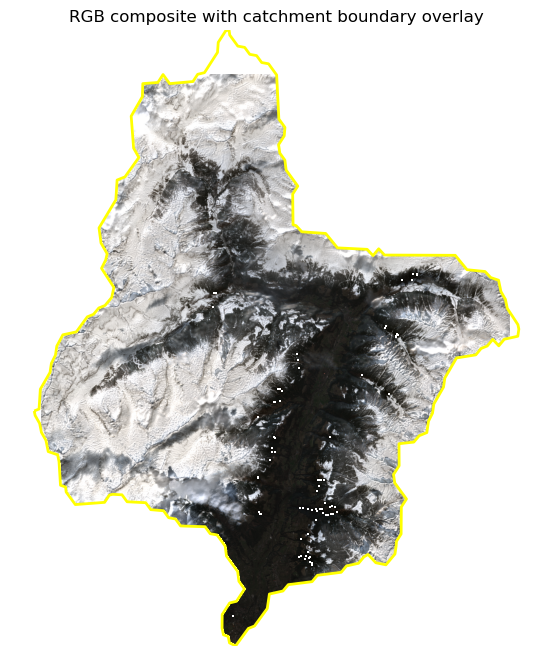
datacubeVisualize area of interest
datacube_sample = datacube.isel(time=15)
rgb = datacube_sample[["b04", "b03", "b02"]].to_dataarray(dim="band")
rgb = rgb.assign_coords(band=["red", "green", "blue"])

vmin = float(rgb.min())
vmax = float(rgb.quantile(0.95))
rgb_scaled = (rgb - vmin) / (vmax - vmin)
rgb_scaled = rgb_scaled.clip(0, 1)

rgb_img = rgb_scaled.transpose("y", "x", "band").values

rgb_img = np.ma.masked_invalid(rgb_img)

x = datacube_sample.x.values
y = datacube_sample.y.values

fig, ax = plt.subplots(figsize=(8, 8))
ax.imshow(rgb_img, extent=[x.min(), x.max(), y.min(), y.max()])

catchment_outline.boundary.plot(ax=ax, edgecolor="yellow", linewidth=2)
ax.set_title("RGB composite with catchment boundary overlay")
ax.axis("off")
plt.show()
/opt/conda/lib/python3.12/site-packages/dask/array/reductions.py:325: RuntimeWarning: All-NaN slice encountered
return np.nanmax(x_chunk, axis=axis, keepdims=keepdims)
Calculate Normalized Difference Snow Index (NDSI)
The Normalized Difference Snow Index (NDSI) is computed as:
ndsi = (datacube["b03"] - datacube["b11"]) / (datacube["b03"] + datacube["b11"])
ndsi = ndsi.rename("ndsi")
ndsiCreate snow map
To create a binary snow map, we apply a threshold to the NDSI values. Pixels with NDSI values greater than 0.4 are classified as snow-covered (1), while those with NDSI values less than or equal to 0.4 are classified as non-snow-covered (0).
ndsi_mask = ndsi > 0.42
snowmap = ndsi_mask.rename("snow_map").where(no_data_mask)
snowmapCreate and apply cloud mask
Using the SCL band from Sentinel-2, we create a cloud mask to filter out cloudy pixels from our snow map.
cloud_mask = datacube["scl"].isin([3, 8, 9])
snowmap_cloudfree = snowmap.where(~cloud_mask, other=2)
snowmap_cloudfreeVisualize timeseries step
snowmap_1d = snowmap_cloudfree.sel(time=slice("2018-02-10", "2018-02-12"))
fig, ax = plt.subplots(figsize=(10, 8))
snowmap_1d.isel(time=0).plot(ax=ax, cmap="viridis")
ax.set_title(f"Snow Map - {snowmap_1d.time.values[0]}")
plt.show()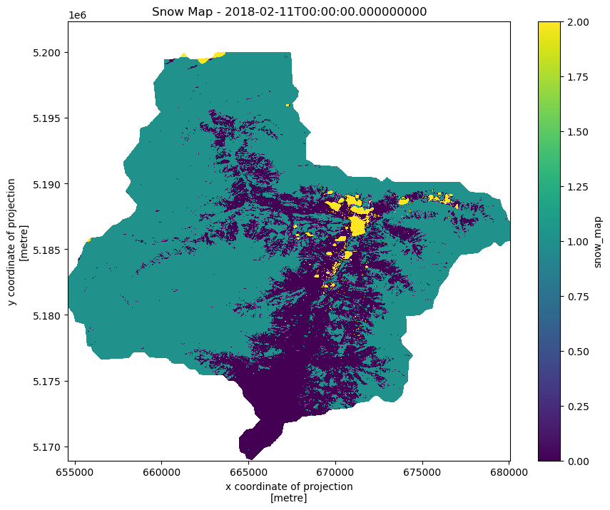
Calculate catchment statistics
We calculate the cloud percentage for the catchment for each timestep. We use this information to filter the timeseries. All timesteps that have a cloud coverage of over 25% will be discarded.
Ultimately we are interested in the snow covered area (SCA) within the catchment. We count all snow covered pixels within the catchment for each time step. Multiplied by the pixel size that would be the snow covered area. Divided the pixel count by the total number of pixels in the catchment is the percentage of pixels covered with snow. We will use this number.
snow_pixels = (snowmap_cloudfree == 1).where(no_data_mask)
cloud_pixels = cloud_mask.where(no_data_mask)
valid_pixels = (snowmap_cloudfree >= 0).where(no_data_mask)

pixel_maps = xr.Dataset(
    {
        "snow_pixels": snow_pixels,
        "cloud_pixels": cloud_pixels,
        "valid_pixels": valid_pixels,
    }
)
catchment_stats = pixel_maps.sum(dim=["x", "y"])
print("Catchment statistics over time:")
print(catchment_stats)
total_pixels = catchment_stats["valid_pixels"]
snow_percentage = catchment_stats["snow_pixels"] / total_pixels * 100
cloud_percentage = catchment_stats["cloud_pixels"] / total_pixels * 100
catchment_stats = catchment_stats.assign(
snow_percentage=snow_percentage, cloud_percentage=cloud_percentage
).compute()Catchment statistics over time:
<xarray.Dataset> Size: 1kB
Dimensions: (time: 40)
Coordinates:
* time (time) datetime64[ns] 320B 2018-02-03 ... 2018-06-26
spatial_ref int64 8B 0
Data variables:
snow_pixels (time) float64 320B dask.array<chunksize=(1,), meta=np.ndarray>
cloud_pixels (time) float64 320B dask.array<chunksize=(1,), meta=np.ndarray>
valid_pixels (time) float64 320B dask.array<chunksize=(1,), meta=np.ndarray>
/opt/conda/lib/python3.12/site-packages/dask/_task_spec.py:759: RuntimeWarning: divide by zero encountered in divide
  return self.func(*new_argspec)
/opt/conda/lib/python3.12/site-packages/dask/_task_spec.py:759: RuntimeWarning: divide by zero encountered in divide
  return self.func(*new_argspec)
/opt/conda/lib/python3.12/site-packages/dask/_task_spec.py:759: RuntimeWarning: divide by zero encountered in divide
  return self.func(*new_argspec)
/opt/conda/lib/python3.12/site-packages/dask/_task_spec.py:759: RuntimeWarning: divide by zero encountered in divide
  return self.func(*new_argspec)
/opt/conda/lib/python3.12/site-packages/dask/_task_spec.py:759: RuntimeWarning: divide by zero encountered in divide
  return self.func(*new_argspec)
/opt/conda/lib/python3.12/site-packages/dask/_task_spec.py:759: RuntimeWarning: divide by zero encountered in divide
  return self.func(*new_argspec)
/opt/conda/lib/python3.12/site-packages/dask/_task_spec.py:759: RuntimeWarning: divide by zero encountered in divide
  return self.func(*new_argspec)
/opt/conda/lib/python3.12/site-packages/dask/_task_spec.py:759: RuntimeWarning: divide by zero encountered in divide
  return self.func(*new_argspec)
/opt/conda/lib/python3.12/site-packages/dask/_task_spec.py:759: RuntimeWarning: divide by zero encountered in divide
  return self.func(*new_argspec)
/opt/conda/lib/python3.12/site-packages/dask/_task_spec.py:759: RuntimeWarning: divide by zero encountered in divide
  return self.func(*new_argspec)
/opt/conda/lib/python3.12/site-packages/dask/_task_spec.py:759: RuntimeWarning: divide by zero encountered in divide
  return self.func(*new_argspec)
/opt/conda/lib/python3.12/site-packages/dask/_task_spec.py:759: RuntimeWarning: divide by zero encountered in divide
  return self.func(*new_argspec)
cloud_threshold = 25

cloud_percent = catchment_stats["cloud_percentage"]

valid_mask = cloud_percent <= cloud_threshold

valid_timesteps = catchment_stats.where(valid_mask, drop=True)

snowmap_filtered = snowmap_cloudfree.where(valid_mask, drop=True)

print("Original timesteps:", len(catchment_stats.time))
print(f"Timesteps with <{cloud_threshold}% clouds:", len(valid_timesteps.time))
Original timesteps: 40
Timesteps with <25% clouds: 22
Plot cloud percentage time series
plt.figure(figsize=(12, 5))

cloud_percent = cloud_percent.assign_coords(
    time=pd.to_datetime(cloud_percent.time.astype("int64"))
)

cloud_percent.plot(marker="o", label="Cloud Percentage")

plt.axhline(y=25, color="r", linestyle="--", label="25% threshold")

plt.title("Cloud Percentage Over Time with Threshold")
plt.ylabel("Cloud Percentage (%)")
plt.xlabel("Time")
plt.legend()
plt.grid(True)

plt.show()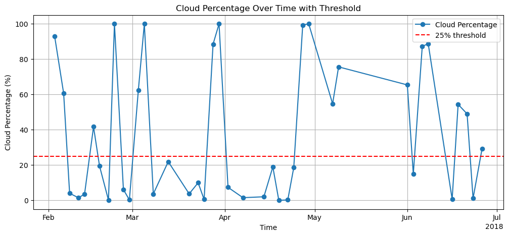
Plot unfiltered snow percentage
snow_percentage = catchment_stats["snow_percentage"]

plt.figure(figsize=(12, 5))

snow_percentage = snow_percentage.assign_coords(
    time=pd.to_datetime(snow_percentage.time.astype("int64"))
)

snow_percentage.plot(marker="o", label="Snow Percentage")

plt.title("Snow Percentage Over Time with Threshold")
plt.ylabel("Snow Percentage (%)")
plt.xlabel("Time")
plt.legend()
plt.grid(True)

plt.show()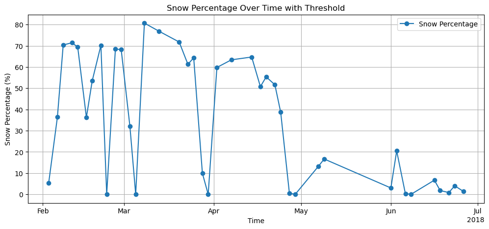
Plot cloud filtered snow percentage
filtered_snow_percentage = snow_percentage.where(valid_mask, drop=True)

filtered_snow_percentage = filtered_snow_percentage.assign_coords(
    time=pd.to_datetime(filtered_snow_percentage.time.astype("int64"))
)

plt.figure(figsize=(12, 5))

filtered_snow_percentage.plot(marker="o", label="Snow Percentage")

plt.title("Cloud-Filtered Snow Percentage Over Time")
plt.ylabel("Snow Percentage (%)")
plt.xlabel("Time")
plt.legend()
plt.grid(True)
plt.show()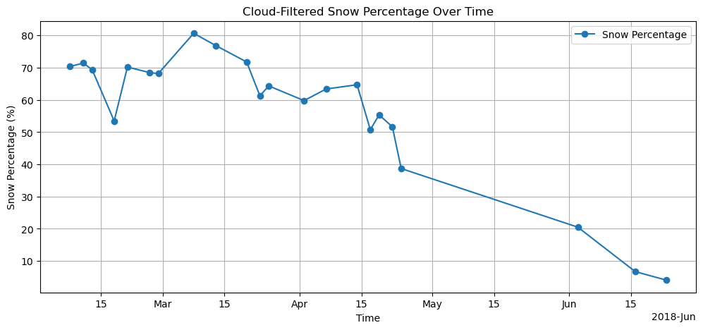
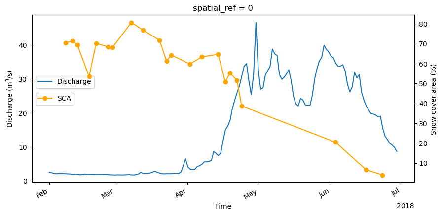
Compare to discharge data
discharge_ds = pd.read_csv(
    "./csv/ADO_DSC_ITH1_0025_CC_31.csv", sep=",", index_col="Time", parse_dates=True
)
discharge_ds.head()Compare the discharge data to the snow covered area.
start_date = datetime(2018, 2, 1)
end_date = datetime(2018, 6, 30)

snow_percent = filtered_snow_percentage.sel(time=slice(start_date, end_date))
discharge_ds = discharge_ds.loc[start_date:end_date]

fig, ax0 = plt.subplots(1, figsize=(10, 5), sharey=True)
ax1 = ax0.twinx()

discharge_ds.discharge_m3_s.plot(
    label="Discharge", ylabel="Discharge (m$^3$/s)", ax=ax0
)
snow_percent.plot(marker="o", ax=ax1, color="orange")

ax0.legend(loc="center left", bbox_to_anchor=(0, 0.6))
ax1.set_ylabel("Snow cover area (%)")
ax1.legend(loc="center left", bbox_to_anchor=(0, 0.5), labels=["SCA"])

plt.show()