EOPF STAC Demo

Author(s): Gisela Romero Candanedo, Julia Wagemann
Affiliation: thriveGEO
Contact: gisela@thrivegeo.com

Introduction¶

In this section, we will dive into the programmatic access of EOPF Zarr Collections available in the EOPF Sentinel Zarr Sample Service STAC Catalog. We will introduce Python libraries that enable us to effectively access and search through STAC.

Disclaimer
This notebook demonstrates the use of open source software and is intended for educational and illustrative purposes only. All software used is subject to its respective licenses. The authors and contributors of this notebook make no guarantees about the accuracy, reliability, or suitability of the content or included code. Use at your own discretion and risk. No warranties are provided, either express or implied.

Table of Contents¶

• 🔹 Setup

• 🔹 Establish a connection to the EOPF Zarr STAC Catalog

• 🔹 Explore available collections

• 🔹 Searching inside the EOPF STAC API

• 🔹 Retrieve Asset URLs for accessing the data

• 🔹 Examining Dataset Structure

• 🔹 Visualising the RGB quicklook composite

• 🔹 Creating our own RGB

• 🔹 Chunking structure

• 🔹 💪 Now it is your turn

• 🔹 Conclusion

Setup¶

For this tutorial, we will make use of the pystac and pystac_client Python libraries that facilitate the programmatic access and efficient search of a STAC Catalog.

Import libraries¶

Helper functions¶

list_found_elements¶

As we are expecting to visualise several elements that will be stored in lists, we define a function that will allow us retrieve item id’s and collections id’s for further retrieval.

normalisation_str_gm()¶

Applies percentile-based contrast stretching and gamma correction to a band.

Recieves:

• band_array : the extracted xarray for the selected band

• p_min : percentile min value

• p_max: percentile max value

• gamma_val: gamma correction

Establish a connection to the EOPF Zarr STAC Catalog¶

Our first step is to establish a connection to the EOPF Sentinel Zarr Sample Service STAC Catalog. For this, you need the Catalog’s base URL, which you can find on the web interface under the API & URL tab. By clicking on 🔗Source, you will get the address of the STAC metadata file - which is available here.

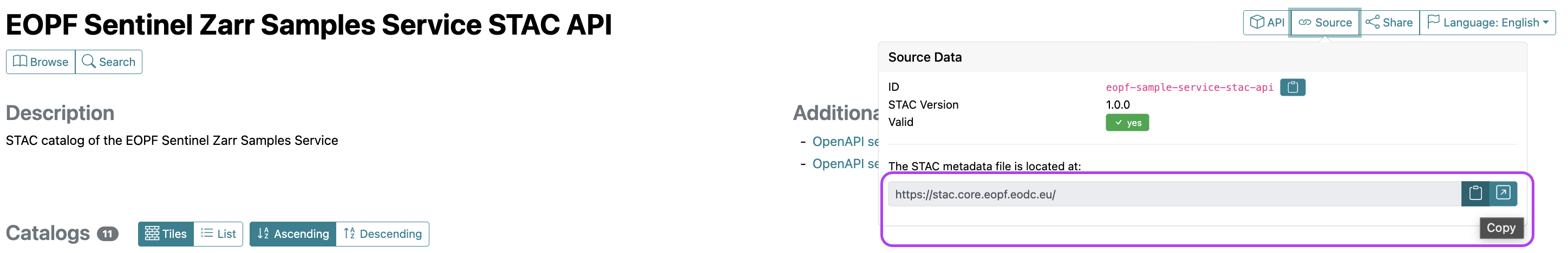
Copy paste the URL: https://stac.core.eopf.eodc.eu/.

With the Client.open() function, we can create the access to the starting point of the Catalog by providing the specific url. If the connection was successful, you will see the description of the STAC catalog and additional information.

Congratulations! We successfully connected to the EOPF Zarr STAC Catalog, and we can now start exploring its content.

Explore available collections¶

Once a connection established, the next logical step is to get an overview of all the collections the STAC catalog offers.

Please note: Since the EOPF Zarr STAC Catalog is still in active development, we need to explore each collection

You see, that so far, we can browse through 11 available collections

We can select any collection and retrieve certain metadata that allow us to get more information about it, such as keywords, the ID and useful links for resources.
For this, we use the .get_collection() argument, and add the corresponding collection id we got earlier.

Sentinel-1 Level-1 GRD¶

Sentinel-2 Level-2A¶

Sentinel-3 SLSTR Level-2 LST¶

Searching inside the EOPF STAC API¶

With the .search() function of the pystac-client library, we can search inside a STAC catalog we established a connection with. We can filter based on a series of parameters to tailor the search for available data for a specific time period and geographic bounding box.

For this, we specify the datetime argument for a time period we are interested in, e.g. from 1st March 2025 to 31st May 2025, over Riga.

Filter for temporal extent¶

Let us search on the datetime parameter. In addition, we also specify the collection parameter indicating that we only want to search for the Sentinel-1 Level-1 GRD collection.

Sentinel-1 Level-1 GRD¶

We apply the helper function list_found_elements which constructs a list from the search result. If we check the length of the final list, we can see that for the specified time period:

Filter for spatial extent¶

Now, let us filter based on a specific area of interest. We can use the bbox argument, which is composed by providing the top-left and bottom-right corner coordinates. It is similar to drawing the extent in the interactive map of the EOPF browser interface.

Sentinel-1 Level-1 GRD¶

For example, we defined a bounding box over Riga. We then again apply the helper function list_found_elements and see:

Sentinel-2 Level-2A¶

Sentinel-3 SLSTR L2 LST¶

Retrieve Asset URLs for accessing the data¶

So far, we have made a search among the STAC catalog and browsed over the general metadata of the collections. To access the actual EOPF Zarr Items, we need to get their storage location in the cloud.

The relevant information we can find inside the .items argument by the .get_assets() function. Inside, it allows us to specify the .MediaType we are interested in. In our example, we want to obtain the location of the .zarr file.

Let us retrieve the url form the available found items form the Sentinel-2 L2A Collection for s2_riga_cloud_search. The resulting URL we can then use to directly access an asset in our workflow.

Examining Dataset Structure¶

In the following step, we open the cloud-optimised Zarr dataset using xarray.open_datatree supported by the zarr engine.

The subsequent loop then prints out all the available groups within the opened DataTree, providing a comprehensive overview of the hierarchical structure of the EOPF Zarr products.

Visualising the RGB quicklook composite¶

EOPF Zarr Assets include a quick-look RGB composite, which we now want to open and visuliase. We open the Zarr dataset again, but this time, we specifically target the quality/l2a_quicklook/r20m/tci.

This group contains a true colour (RGB) quick-look composite, which is a readily viewable representation of the satellite image. By adding .plot.imshow() we can load the quick-look.

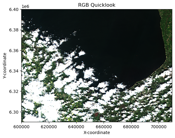
Creating our own RGB¶

For the composite creation, zarr_meas contains the assets we are interested in. The TCI composite makes use of the red (B04), green (B03), and blue (B02) bands to create a view that looks natural to the human eye.

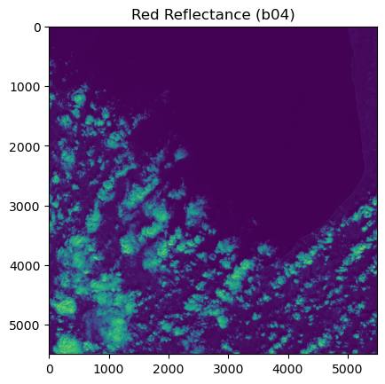
By this point, we have not accessed the data on disk. For doing so, we need to call the .values function from xarray

To create the composite image, we need to normalise each of the input assets. Normalisation ensures that the bands have a consistent and predictable range of values. This supports optimal data processing and removes the influence of external factors (like changing light conditions) allowing for a meaningful comparison among generated composites.

The normalisation_str_gm() function achieves this by scaling the reflectance values to a standard range (0-255) using the percentile-based method.

Once the values for our three bands have been normalised, they can be stacked in an RGB format to generate the initial True Colour Image (TCI).

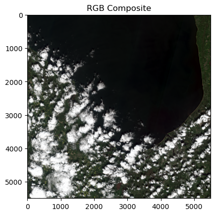
Chunking structure¶

We can have a look at the reflectance values at 20m resolution chunking strategies by adding .chunksizes to the r20m group.

For exploring each of the x and y dimensions, we retrieve the list for each:

We can also explore 10m resolution:

And the same for 60m resolution:

💪 Now it is your turn¶

• Go to the Jupyter Hub

• Clone the GitHub Repo

• Select the 01_intro_stac_task.ipynb version of this notebook.

• Explore this two collections:

Task 1¶

Sentinel-1 Level-1 GRD over Sicily¶

• Starting and ending date:
  2025-05-01 to 2025-05-31

• Bounding box search:
  12.217097,36.537123,15.710750,38.497568

Task 2¶

Sentinel-2 L-2A over Vienna¶

• Starting and ending date:
  2025-04-01 to 2025-04-30

• Bounding box search:
  16.126524,48.096899,16.660573,48.316752

Explore...¶

• How many items are available?

• Filter the cloud percentage... How many items are still available?

• Recreate an RGB composite for Sentinel-2 L-2A over Vienna.

Conclusion¶

In this section we established a connection to the EOPF Sentinel Zarr Sample Service STAC Catalog and directly accessed an EOPF Zarr item with xarray. In the tutorial you are guided through the process of opening hierarchical EOPF Zarr products using xarray’s DataTree, a library designed for accessing complex hierarchical data structures.
We also brought data to disk and processed it to obtain an RGB composite, always highlighting the flexibility of data retrieval through STAC and the zarr format.

What’s Next?¶

In the following section we will explore the application of an RBG composite creation a True Colour Image from Sentinel-2 L2A data for the day of the fire.

To obtain a more detailed overview of a natural event, we will integrate an additional dataset into our workflow: Sentinel-3 data. This will enable us to analyse thermal information and pinpoint the active fire’s location.