Dask Intro - Welcome

Dask Introduction¶

Run this notebook interactively with all dependencies pre-installed

Table of Contents¶

Introduction
Imports
Setup
Cluster
Workflow
Cleanup
Summary

Introduction¶

This notebook demonstrates how to open, explore, and visualize Sentinel-1 GRD products stored in EOPF Zarr format, including accessing, geocoding, subsetting and plotting a single polarization.

Import Modules¶

from dask_gateway import Gateway

Setup¶

The setup is very simple, you will just need the following lines. Each of our JupyterLab instances starts with the gatway data preconfigured.

"""
gate = Gateway("https://dask.user.eopf.eodc.eu",
               proxy_address="tls://dask.user.eopf.eodc.eu:10000",
               auth="jupyterhub")
"""

# Dask Gateway automatically loads the correct configuration.
# So the code below is identical to the comment above
gate = Gateway()

Cluster Options / Custom image¶

Before spinning up a cluster you can also define your ‘cluster_options’, allowing you to define a custom image for your dask cluster.

# Define cluster options
cluster_options = gate.cluster_options()

# Specify the Docker image to use for the workers
cluster_options.image = "repository.io/organisation/cluster_image:tag"

# Create a new cluster with the specified options
cluster = gate.new_cluster(cluster_options)
cluster

If you want to use the default image you can just use this code.

cluster = gate.new_cluster()
cluster

Cluster Object¶

When running the lines above, you’ll be presented with the following interface:

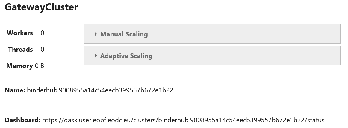
This UI allows you to quickly scale the amount of workers you need.

Alternatively you can also use the following lines of code for scaling:

cluster.scale(2)

cluster.adapt(minimum=1, maximum=2)

Cluster options allow you to

Next, you’ll have to create a dask client object, this is the last step before we can start working with our cluster.

client = cluster.get_client()

client

This should also give you an url giving you access to your Dask Dashboard.
This gives you an overview of the workers and workloads in your dask cluster.
There’s also a JupyterHub Extension giving you the same overview inside of your JupyterLab.

¶

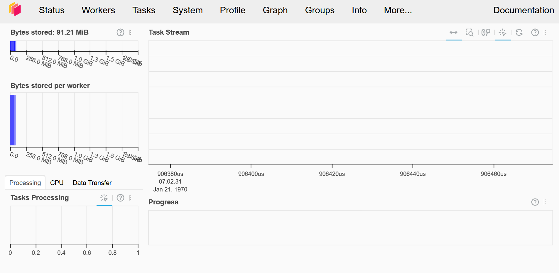
The following code-blocks outline a rudimentary workflow to get you going with Dask.

Here we create an array of random numbers, add it to its own transposition and then calculate the mean across a slice of the data.

import dask.array as da

x = da.random.random((10000, 10000), chunks=(1000, 1000))

y = x + x.T
z = y[::2, 5000:].mean(axis=1)
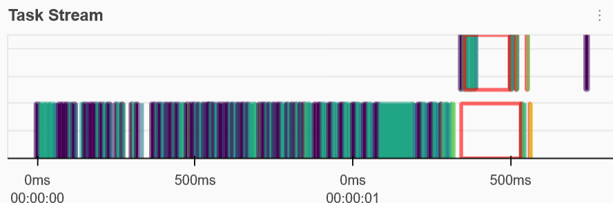
z

Until now this has all been done lazily, in order to actually get our results

result = z.compute()

In your dashboard you will see the task stream filling up, and once the computation is done you can keep using the resulting data locally.

Cleanup¶

Make sure to shut down your cluster when you’re done working with it.

cluster.shutdown()

Summary¶

This notebook explained how to interact with the Dask services available through the EOPF Sample Service.