NDSI based snow mapping with Sentinel-2

Table of Contents¶

Introduction
Import modules
False Color Composite Visualization
Cloud Masking
NDSI Computation
Snow Map Visualization

Run this notebook interactively with all dependencies pre-installed

Introduction¶

Snow monitoring plays a crucial role in water resource management 💧. The increasing availability of remote sensing data 🛰️ offers significant advantages, but also introduces challenges related to data accessibility, processing, and storage. For operational use, scalable workflows are essential to ensure global applicability. Leveraging a cloud-native format like EOPF Zarr enables to get a quick prototype ready before scaling it up in the cloud, for instance using the openEO API. The workflow is built using the EOPF Zarr Samples STAC API, in combination with the xcube-eopf plugin, which enables us to build data cubes directly from STAC.
If you want to know more detila about the usage of the xcube-eopf plugin, please refer to the Introduction to xcube-eopf Data Store notebook.

Import Modules¶

The xcube-eopf data store is implemented as a plugin for xcube. Once installed, it registers the store ID eopf-zarr automatically and a new data store instance can be initiated via xcube’s new_data_store() method.

from xcube.core.store import new_data_store
from xcube_eopf.utils import reproject_bbox

import matplotlib.pyplot as plt
from matplotlib.colors import ListedColormap
from matplotlib.patches import Patch

import numpy as np

store = new_data_store("eopf-zarr")

Data Access¶

We firstly define the parameters that will be used to query the EOPF Sentinel Zarr Samples STAC API.
The Area Of Interest (AOI) covers part of the Oetztal Alps, between South Tyrol (Italy) and Tyrol (Austria).
We will work on a single image, which is almost cloud-free, but you could easily extend the example to multiple dates.

bbox = [10.6, 46.74, 11, 46.91]
crs_utm = "EPSG:32632"
bbox_utm = reproject_bbox(bbox, "EPSG:4326", crs_utm)

Pass the parameters to the xcube plugin and create the datacube.

💡 Note
open_data() builds a Dask graph and returns a lazy xarray.Dataset. No actual data is loaded at this point. The data is loaded as reflectances, i.e. with the offset and scale factors already applied.

ds = store.open_data(
    data_id="sentinel-2-l2a",
    bbox=bbox_utm,
    time_range=["2025-06-18", "2025-06-20"],
    spatial_res=10,
    crs=crs_utm,
    variables=["b02", "b03", "b04", "b08", "b11", "scl"],
)
ds

False Color Composite Visualization¶

Let’s visualize a false color composite (R: SWIR, G: NIR, B: RED) and the classic RGB side by side.
In this case, you can notice that false color composite enhances the visibility of snow-covered areas compared to clouds.
Before the visualization, we rescale the data to improve the visibility.

false_color_composite = (
    (ds[["b11", "b08", "b04"]].to_dataarray(dim="bands") / 0.7)
    .clip(0, 1)
    .squeeze("time")
    .transpose("y", "x", "bands")
)
rgb_composite = (
    (ds[["b04", "b03", "b02"]].to_dataarray(dim="bands") / 0.25)
    .clip(0, 1)
    .squeeze("time")
    .transpose("y", "x", "bands")
)

fig, ax = plt.subplots(figsize=(15, 6))
ax.axis("off")
plt.subplot(121)
plt.axis("off")
plt.title("Sentinel-2 false color composite (R:SWIR,G:NIR,B:RED)")
plt.imshow(false_color_composite)
plt.subplot(122)
plt.axis("off")
plt.title("Sentinel-2 RGB color composite")
plt.imshow(rgb_composite)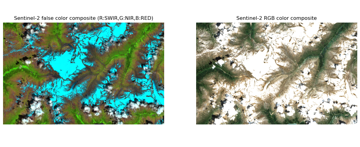

/home/mclaus@eurac.edu/micromamba/envs/eopf-zarr3/lib/python3.11/site-packages/numpy/core/numeric.py:407: RuntimeWarning: invalid value encountered in cast
  multiarray.copyto(res, fill_value, casting='unsafe')
/home/mclaus@eurac.edu/micromamba/envs/eopf-zarr3/lib/python3.11/site-packages/numpy/core/numeric.py:407: RuntimeWarning: invalid value encountered in cast
  multiarray.copyto(res, fill_value, casting='unsafe')

Cloud Masking¶

As usual, we mask out the clouds before proceeding in our snow mapping workflow.

valid_mask = np.logical_not(ds["scl"].isin([8, 9, 3]))

ds_valid = ds.where(valid_mask)

false_color_composite_masked = false_color_composite.where(valid_mask[0])

NDSI Computation¶

❄️ To rapidly classify snow-covered areas, we calculate the Normalized Difference Snow Index (NDSI) using the shortwave infrared (SWIR) and green bands:

NDSI=\frac {GREEN-SWIR}{GREEN+SWIR}

(1)

This normalized difference highlights snow by taking advantage of its high reflectance in the green band and strong absorption in the SWIR band.

green = ds_valid["b03"]
swir = ds_valid["b11"]

ndsi = (green - swir) / (green + swir)

snow_map = ndsi > 0.42

snow_map

Snow Map Visualization¶

Let’s visualize the classification output and compare it with the cloud-masked false color composite.

fig, axes = plt.subplots(1, 2, figsize=(10, 5))

# Plot RGB image
axes[0].imshow(false_color_composite_masked)
axes[0].axis("off")
axes[0].set_title("Sentinel-2 False Color Composite\n(R: SWIR, G: NIR, B: RED)")

# Plot binary snow classification
binary_data = snow_map.squeeze("time")

# Define discrete colormap: 0 = no snow (light gray), 1 = snow (blue)
cmap = ListedColormap(["brown", "cyan"])

im = axes[1].imshow(binary_data, cmap=cmap)
axes[1].axis("off")
axes[1].set_title("Snow Classification (NDSI threshold)")

# Create custom legend
legend_elements = [
    Patch(facecolor="brown", edgecolor="k", label="Snow-free"),
    Patch(facecolor="cyan", edgecolor="k", label="Snow"),
]

axes[1].legend(handles=legend_elements, loc="lower right")

plt.tight_layout()
plt.show()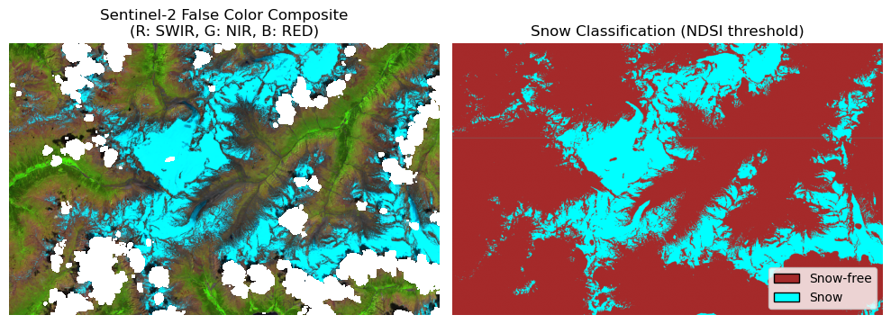

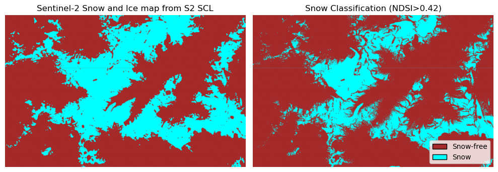
Finally, let’s compare our snow map with the Scene Classification Layer (SCL) shipped with the Sentinel-2 L2A data:

scl_snow_ice_map = ds.scl == 11
scl_snow_ice_map

fig, axes = plt.subplots(1, 2, figsize=(10, 5))

# Define discrete colormap: 0 = no snow (light gray), 1 = snow (blue)
cmap = ListedColormap(["brown", "cyan"])

# Plot SCL Snow and Ice map
axes[0].imshow(scl_snow_ice_map.squeeze("time"), cmap=cmap)
axes[0].axis("off")
axes[0].set_title("Sentinel-2 Snow and Ice map from S2 SCL")

# Plot binary snow classification
binary_data = snow_map.squeeze("time")

im = axes[1].imshow(binary_data, cmap=cmap)
axes[1].axis("off")
axes[1].set_title("Snow Classification (NDSI>0.42)")

# Create custom legend
legend_elements = [
    Patch(facecolor="brown", edgecolor="k", label="Snow-free"),
    Patch(facecolor="cyan", edgecolor="k", label="Snow"),
]

axes[1].legend(handles=legend_elements, loc="lower right")

plt.tight_layout()
plt.show()

Welcome

STAC-Based Exploration and Visualization of Sentinel-2 and Sentinel-1 Data

Welcome

Sentinel Data