Introduction to xcube-eopf Data Store.
A xcube Data Store providing Analysis-Ready Datacubes (ARDC) from EOPF Sentinel Zarr Samples
Table of Contents
Run this notebook interactively with all dependencies pre-installed
Introduction
xcube-eopf is a Python package and xcube plugin that adds a data store named eopf-zarr to xcube. The data store is used to provide analysis-ready datacubes (ARDC) from EOPF Sentinel Zarr Samples.
This notebook demonstrates how to use the xcube-eopf plugin to explore and analyze EOPF Sentinel Zarr Samples. It highlights the key features currently supported by the plugin.
- 🐙 GitHub: EOPF Sample Service – xcube-eopf
- ❗ Issue Tracker: Submit or view issues
- 📘 Documentation: xcube-eopf Docs
Install the xcube-eopf Data Store
The xcube-eopf package is implemented as a xcube plugin and can be installed using either pip or conda/mamba from the conda-forge channel.
📦 PyPI: xcube-eopf on PyPI
pip install xcube-eopf🐍 Conda (conda-forge): xcube-eopf on Anaconda
conda install -c conda-forge xcube-eopfYou can also use Mamba as a faster alternative to Conda:
mamba install -c conda-forge xcube-eopf
Introduction to xcube
xcube is an open-source Python toolkit for transforming Earth Observation (EO) data into analysis-ready datacubes following CF conventions. It enables efficient data access, processing, publication, and interactive exploration.
Key components of xcube include:
- xcube data stores – efficient access to EO datasets
- xcube data processing – creation of self-contained analysis-ready datacubes
- xcube Server – RESTful APIs for managing and serving data cubes
- xcube Viewer – a web app for visualizing and exploring data cubes
Data Stores
Data stores are implemented as plugins. Once installed, it registers automatically and can be accessed via xcube’s new_data_store() method. The most important operations of a data store instance store are:
store.list_data_ids()- List available data sources.store.has_data(data_id)- Check data source availability.store.get_open_data_params_schema(data_id)- View available open parameters for each data source.store.open_data(data_id, **open_params)- Open a given dataset and return, e.g., an xarray.Dataset instance.
To explore all available functions, see the Python API.
Main Features of the xcube-eopf Data Store
The xcube-eopf plugin uses the xarray-eopf backend to access individual EOPF Zarr samples, then leverages xcube’s data processing capabilities to generate a 3D analysis-ready datacube (ARDCs) from multiple samples.
Currently, this functionality supports Sentinel-2 products.
The workflow for building datacubes from multiple Sentinel-2 products involves the following steps, which are implemented in the open_data() method:
- Query products using the EOPF STAC API for a given time range and spatial extent.
- Retrieve observations as cloud-optimized Zarr chunks via the xarray-eopf backend (Webinar 3).
- Mosaic spatial tiles into single images per timestamp.
- Stack the mosaicked scenes along the temporal axis to form a 3D cube.
📚 More info: xcube-eopf Documentation
Import Modules
The xcube-eopf data store is implemented as a plugin for xcube. Once installed, it registers the store ID eopf-zarr automatically and a new data store instance can be initiated via xcube’s new_data_store() method.
import os

import dask
import xarray as xr
from xcube.core.store import new_data_store
from xcube.util.config import load_configs
from xcube.webapi.viewer import Viewer
from xcube_eopf.utils import reproject_bboxxr.set_options(display_expand_attrs=False)<xarray.core.options.set_options at 0x7f5897571160>store = new_data_store("eopf-zarr")Data Store Basics
The following section introduces the basic functionality of an xcube data store. It helps you navigate the store and identify the appropriate parameters for opening datacubes.
The data IDs point to STAC collections. So far 'sentinel-2-l1c' and 'sentinel-2-l2a' is supported. To list all available data IDs:
store.list_data_ids()['sentinel-2-l1c', 'sentinel-2-l2a']One can also check if a data ID is available via the has_data() method, as shown below:
store.has_data("sentinel-2-l2a")TrueThe Sentinel-1 GRD product is not yet available, so the following cell returns False:
store.has_data("sentinel-1-l1-grd")FalseBelow, you can view the parameters for the open_data() method for each supported data product. The following cell generates a JSON schema that lists all opening parameters for each supported Sentinel product.
store.get_open_data_params_schema()Open Multiple Sentinel-2 Samples as an Analysis-Ready Data Cube
Sentinel-2 provides multi-spectral imagery at varying native spatial resolutions:
- 10m:
b02,b03,b04,b08 - 20m:
b05,b06,b07,b8a,b11,b12 - 60m:
b01,b09,b10
Sentinel-2 products are organized as STAC Items, each representing a single tile. These tiles overlap and are stored in their native UTM coordinate reference system (CRS), which varies by geographic location.
Data Cube Generation Workflow
- STAC Query: A STAC API request returns relevant STAC Items (tiles) based on
spatial and temporal extent (
bboxandtime_rangeargument). - Sorting: Items are ordered by solar acquisition time and Tile ID.
- Native Alignment: Within each UTM zone, tiles from the same solar day are aligned in the native UMT without reprojection. Overlaps are resolved by selecting the first non-NaN pixel value in item order.
- Cube Assembly: The method of cube creation depends on the user’s request, as summarized below:
| Scenario | Native Resolution Preservation | Reprojected or Resampled Cube |
|---|---|---|
| Condition | Requested bounding box lies within a single UTM zone, native CRS is requested, and the spatial resolution matches the native resolution. | Data spans multiple UTM zones, a different CRS is requested (e.g., EPSG:4326), or a custom spatial resolution is requested. |
| Processing steps | Only upsampling or downsampling is applied to align the differing resolutions of the spectral bands. Data cube is directly cropped using the requested bounding box, preserving original pixel values. Spatial extent may deviate slightly due to alignment with native pixel grid. | A target grid mapping is computed from bounding box, spatial resolution, and CRS. Data from each UTM zone is reprojected/resampled to this grid. Overlaps resolved by first non-NaN pixel. |
The get_open_data_params_schema(data_id) function can also be used for a specific data_id. It provides descriptions of the available opening parameters, including their format and whether they are required.
When calling open_data(data_id, **open_params), the provided parameters are validated against this schema. If they do not match, an error is raised immediately.
store.get_open_data_params_schema(data_id="sentinel-2-l2a")Below the opening parameters for the Sentinel-2 product (applicable for L1C and L2A) are summarized:
Required parameters:
bbox: Bounding box [“west”, “south”, “est”, “north”] in CRS coordinates.time_range: Temporal extent [“YYYY-MM-DD”, “YYYY-MM-DD”].spatial_res: Spatial resolution in meter of degree (depending on the CRS).crs: Coordinate reference system (e.g."EPSG:4326").
These parameters control the STAC API query and define the output cube’s spatial grid.
Optional parameters:
variables: Variables to include in the dataset. Can be a name or regex pattern or iterable of the latter.- Surface reflectance bands:
b01,b02,b03,b04,b05,b06,b07,b08,b8a,b09,b11,b12 - Classification/Quality layers (L2A only):
cld,scl,snw
- Surface reflectance bands:
tile_size: Spatial tile size of the returned dataset(width, height).query: Additional query options for filtering STAC Items by properties. See STAC Query Extension for details.spline_orders: governs 2D interpolation; accepts a single order for all variables, or a dictionary mapping orders to variable names or data types; Supported spline orders:0: nearest neighbor (default forscl)1: linear2: bi-linear3: cubic (default)
agg_methods: governs the aggregation method during downsampling; accepts a single order for all variables, or a dictionary mapping orders to variable names or data types. Supported spline orders:"mean"(default)"center"(default forscl)"count","first","last","max","median","mode","min","prod","std","sum","var"
We now want to generate a small example data cube in native UTM projection from the Sentinel-2 L2A samples:
- Assign
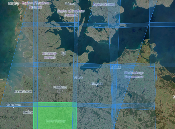
data_idto"sentinel-2-l2a". - Set the bounding box to cover Hamburg area.
- Set the time range to the first week of Mai 2025.
bbox = [9.85, 53.5, 10.05, 53.6]
crs_utm = "EPSG:32632"
bbox_utm = reproject_bbox(bbox, "EPSG:4326", crs_utm)
💡 Noteopen_data() builds a Dask graph and returns a lazy xarray.Dataset. No actual data is loaded at this point.
%%time
ds = store.open_data(
    data_id="sentinel-2-l2a",
    bbox=bbox_utm,
    time_range=["2025-05-01", "2025-05-07"],
    spatial_res=10,
    crs=crs_utm,
    variables=["b02", "b03", "b04", "scl"],
)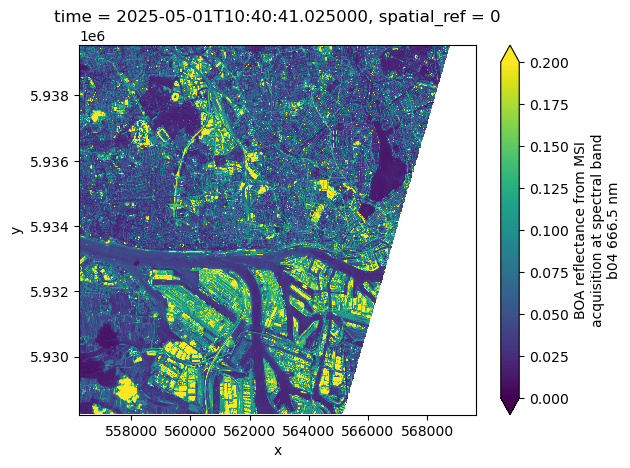
dsWe can plot the the red band (b04) for the first time step as an example. This operation triggers data downloads and processing.
%%time
ds.b04.isel(time=0).plot(vmin=0, vmax=0.2)
CPU times: user 231 ms, sys: 72.7 ms, total: 304 ms
Wall time: 450 ms
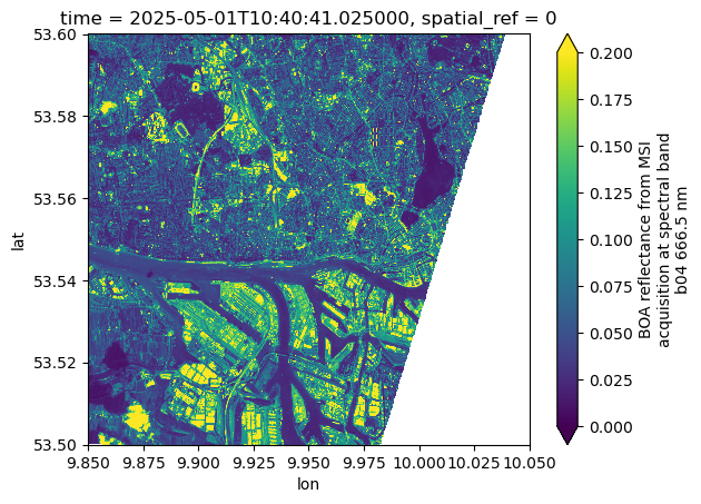
Now we can request the same data cube but in geographic projection (“EPSG:4326”). xcube-eopf can reproject the datacube to any projection requested by the user.
%%time
ds = store.open_data(
    data_id="sentinel-2-l2a",
    bbox=bbox,
    time_range=["2025-05-01", "2025-05-07"],
    spatial_res=10 / 111320,  # meters converted to degrees (approx.)
    crs="EPSG:4326",
    variables=["b02", "b03", "b04", "scl"],
)
ds%%time
ds.b04.isel(time=0).plot(vmin=0, vmax=0.2)CPU times: user 897 ms, sys: 99.4 ms, total: 996 ms
Wall time: 967 ms
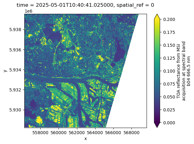
We now want to generate a similar data cube from the Sentinel-2 L1C product. We therefore assign data_id to "sentinel-2-l1c".
%%time
ds = store.open_data(
    data_id="sentinel-2-l1c",
    bbox=bbox_utm,
    time_range=["2025-05-01", "2025-05-07"],
    spatial_res=10,
    crs=crs_utm,
    variables=["b02", "b03", "b04"],
)
ds%%time
ds.b04.isel(time=0).plot(vmin=0, vmax=0.2)CPU times: user 226 ms, sys: 23.2 ms, total: 249 ms
Wall time: 365 ms
End-to-End Example: Data Access, Saving, and Visulation
In this example, we retrieve a data cube with a larger spatial extent, covering Mount Etna, and a longer time period, spanning May 2025.
Due to the increased size of this job, we limit Dask parallelization to 4 workers. This ensures a more stable and reliable process when writing the final data cube to the storage.
%%time
dask.config.set(scheduler="threads", num_workers=4)

bbox = [14.8, 37.45, 15.3, 37.85]
crs_utm = "EPSG:32633"
bbox_utm = reproject_bbox(bbox, "EPSG:4326", crs_utm)
ds = store.open_data(
    data_id="sentinel-2-l2a",
    bbox=bbox_utm,
    time_range=["2025-05-01", "2025-06-01"],
    spatial_res=20,
    crs=crs_utm,
    variables=["b02", "scl"],
)
dsSaving the Data Cube
While the EOPF xcube plugin primarily facilitates data access, it also integrates smoothly with the broader xcube ecosystem for post-processing and data persistence.
To save a data cube, you can use the memory xcube data store for in-memory storage — ideal for small examples or demonstrations that don’t require writing to disk.
💡 Note For real-world scenarios, you’ll typically want to persist data cubes to a local filesystem or an S3-compatible object store using the file or s3 backends.
Local Filesystem Data Store:
storage = new_data_store("file")S3 Data Store:
storage = new_data_store(
    "s3",
    root="bucket-name",
    storage_options=dict(
        anon=False,
        key="your_s3_key",
        secret="your_s3_secret",
    ),
)
More info: Filesystem-based data stores.
storage = new_data_store("memory", root="data")We can then persist the retrieved data cube by writing it using the storage data store:
%%time
storage.write_data(ds, "sen2_etna_cube.levels", num_levels=5, replace=True)
/opt/conda/lib/python3.12/site-packages/dask/array/chunk.py:279: RuntimeWarning: invalid value encountered in cast
return x.astype(astype_dtype, **kwargs)
/opt/conda/lib/python3.12/site-packages/dask/array/chunk.py:279: RuntimeWarning: invalid value encountered in cast
return x.astype(astype_dtype, **kwargs)
CPU times: user 41 s, sys: 2.31 s, total: 43.3 s
Wall time: 53.6 s
'sen2_etna_cube.levels'This writes the final data cube in a custom multi-resolution Zarr format, referred to as the levels format. It is conceptually similar to Cloud-Optimized GeoTIFF (COG) but based on Zarr layers.
The num_levels parameter controls how many lower-resolution levels are generated. Each additional level reduces the spatial resolution by a factor of two, which is particularly useful for efficient visualization and zooming in the xcube Viewer app.
Visualization and Analysis
💡 Note
If you are running this notebook on the EOPF Sample Service JupyterHub, please set the following environment variable to ensure the Viewer is configured with the correct endpoint.
The environment variable should be set to: "https://jupyterhub.user.eopf.eodc.eu/user/<E-mail>/"
Replace <E-mail> with the email address you use to log in to CDSE. This corresponds to the first part of the URL displayed in your browser after logging into JupyterHub.
os.environ["XCUBE_JUPYTER_LAB_URL"] = (
    "https://jupyterhub.user.eopf.eodc.eu/user/konstantin.ntokas@brockmann-consult.de/"
)
Once saved as levels to the storage data store, we can open the multi-resolution datacube and open the base layer with the original resolution of 20m.
mlds = storage.open_data("sen2_etna_cube.levels")
ds = mlds.get_dataset(0)
dsNext we use xcube Viewer to visualize the cube. The Viewer can be configured via a yaml file. The info() method gives the URL of the Viewer instance which can be used to open the web application.
config = load_configs("server_config.yaml")
viewer = Viewer(server_config=config)
viewer.info()
Server: https://jupyterhub.user.eopf.eodc.eu/user/konstantin.ntokas@brockmann-consult.de/proxy/8000
Viewer: https://jupyterhub.user.eopf.eodc.eu/user/konstantin.ntokas@brockmann-consult.de/proxy/8000/viewer/?serverUrl=https://jupyterhub.user.eopf.eodc.eu/user/konstantin.ntokas@brockmann-consult.de/proxy/8000
404 GET /viewer/config/config.json (127.0.0.1): xcube viewer has not been been configured
404 GET /viewer/config/config.json (127.0.0.1) 5.90ms
501 GET /viewer/state?key=sentinel (127.0.0.1) 0.52ms
404 GET /viewer/ext/contributions (127.0.0.1) 136.38ms
The Viewer can also be opened within the Jupyter notebook:
viewer.show()Alternative: visualize datasets in xcube Viewer via Python API
Alternatively, the viewer can be started via the Python API. Here, the desired data cubes are added to the viewer via the method add_dataset().
viewer = Viewer()
viewer.add_dataset(ds)
viewer.show()Conclusion
This notebook demonstrates the current development status of the xcube-eopf data store, which adds a data store named eopf-zarr to the xcube framework. Below is a summary of the key takeaways:
- 3D analysis-ready spatio-temporal data cubes can be generated from multiple EOPF Sentinel Zarr samples (currently limited to Sentinel-2).
- The cube generation workflow follows this pattern:
- Query via the EOPF STAC API
- Read using the xarray-eopf backend (Webinar 3)
- Mosaic along spatial axes
- Stack along the time axis
- The end-to-end workflow with xcube includes:
- Data access via the
eopf-zarrdata store - Cube persistence using writable data stores (
file,s3) - Visualization using xcube Viewer
- Data access via the
Future Development
- Extend support to include Sentinel-1 and Sentinel-3 data.
- Incorporate user feedback — please test the plugin and report issues here: 👉 GitHub Issues – xcube-eopf
- Continue active development of the plugin through January 2026, at least within the scope of the EOPF Sentinel Zarr Samples project.
