Sentinel-1 GRD Zarr Product Exploration

Sentinel-1 GRD Zarr Product Exploration¶

Table of Contents¶

Introduction
Import modules
File path definition
Open the product
Overview of the product content
Explore product geolocation
Data Decimation
Geocoding using GCPs
Geographic selection
Summary

Introduction¶

This notebook demonstrates how to open, explore, and visualize Sentinel-1 GRD products stored in EOPF Zarr format, including accessing, geocoding, subsetting and plotting a single polarization.

Import Modules¶

import xarray as xr
import matplotlib.pyplot as plt
import cartopy.crs as ccrs

xr.set_options(display_expand_attrs=False)
plt.rcParams["figure.figsize"] = (10, 5)
plt.rcParams["font.size"] = 10

File path definition¶

GRD: S1A_IW_GRDH_1SDV_20170508T164830_20170508T164855_016493_01B54C_8604

polarization: VH

product = "S1A_IW_GRDH_1SDV_20170508T164830_20170508T164855_016493_01B54C_8604"
remote_product_path = f"https://objectstore.eodc.eu:2222/e05ab01a9d56408d82ac32d69a5aae2a:sample-data/tutorial_data/cpm_b716/{product}.zarr"

Open the product¶

The GRD product can be opened as a DataTree using Xarray:

dt = xr.open_datatree(remote_product_path, engine="zarr", chunks={})
dt

Overview of the product content¶

The Zarr GRD product contains one group for each polarization:

dt.groups[1]

'/S01SIWGRD_20170508T164830_0025_A094_8604_01B54C_VH'

Each polarization group contains the conditions, measurements and quality groups. We can list all the groups for the VH polarization calling .groups

dt[dt.groups[1]].groups

('/S01SIWGRD_20170508T164830_0025_A094_8604_01B54C_VH',
 '/S01SIWGRD_20170508T164830_0025_A094_8604_01B54C_VH/conditions',
 '/S01SIWGRD_20170508T164830_0025_A094_8604_01B54C_VH/measurements',
 '/S01SIWGRD_20170508T164830_0025_A094_8604_01B54C_VH/quality',
 '/S01SIWGRD_20170508T164830_0025_A094_8604_01B54C_VH/conditions/antenna_pattern',
 '/S01SIWGRD_20170508T164830_0025_A094_8604_01B54C_VH/conditions/attitude',
 '/S01SIWGRD_20170508T164830_0025_A094_8604_01B54C_VH/conditions/azimuth_fm_rate',
 '/S01SIWGRD_20170508T164830_0025_A094_8604_01B54C_VH/conditions/coordinate_conversion',
 '/S01SIWGRD_20170508T164830_0025_A094_8604_01B54C_VH/conditions/doppler_centroid',
 '/S01SIWGRD_20170508T164830_0025_A094_8604_01B54C_VH/conditions/gcp',
 '/S01SIWGRD_20170508T164830_0025_A094_8604_01B54C_VH/conditions/orbit',
 '/S01SIWGRD_20170508T164830_0025_A094_8604_01B54C_VH/conditions/reference_replica',
 '/S01SIWGRD_20170508T164830_0025_A094_8604_01B54C_VH/conditions/replica',
 '/S01SIWGRD_20170508T164830_0025_A094_8604_01B54C_VH/conditions/terrain_height',
 '/S01SIWGRD_20170508T164830_0025_A094_8604_01B54C_VH/quality/calibration',
 '/S01SIWGRD_20170508T164830_0025_A094_8604_01B54C_VH/quality/noise',
 '/S01SIWGRD_20170508T164830_0025_A094_8604_01B54C_VH/quality/noise_range')

Access now the VH polarization group and the GRD DataArray

grd = dt[dt.groups[1]]["measurements/grd"]
grd

Explore product geolocation¶

The Zarr product metadata contains information about the product geolocation we can explore in various ways. For instance, we can show the product footprint on an interactive map.

import geopandas as gpd

# Create a GeoDataFrame from the feature
gdf = gpd.GeoDataFrame.from_features(
    [
        {
            "type": "Feature",
            "geometry": dt.attrs["stac_discovery"][
                "geometry"
            ],  # Use the actual geometry, not the bbox
            "properties": dt.attrs["stac_discovery"][
                "properties"
            ],  # Include all properties
        }
    ],
    crs="EPSG:4326",  # Set the CRS explicitly (adjust EPSG code if needed)
)
gdf.explore()

Data Decimation¶

We compose a new object, applying decimation to reduce the data we consider for visualization, speeding up the process. Moreover, the original resolution wouldn’t fit on most screens. Decimation is performed using the .isel xarray method. Here we take one pixel every 10 available in the original dataset:

.isel(x=slice(None, None, 10), y=slice(None, None, 10))

# Decimation data
## decimation
grd_decimated = grd.isel(
    azimuth_time=slice(None, None, 10), ground_range=slice(None, None, 10)
)

## plot
grd_decimated.plot(vmax=200)
plt.show()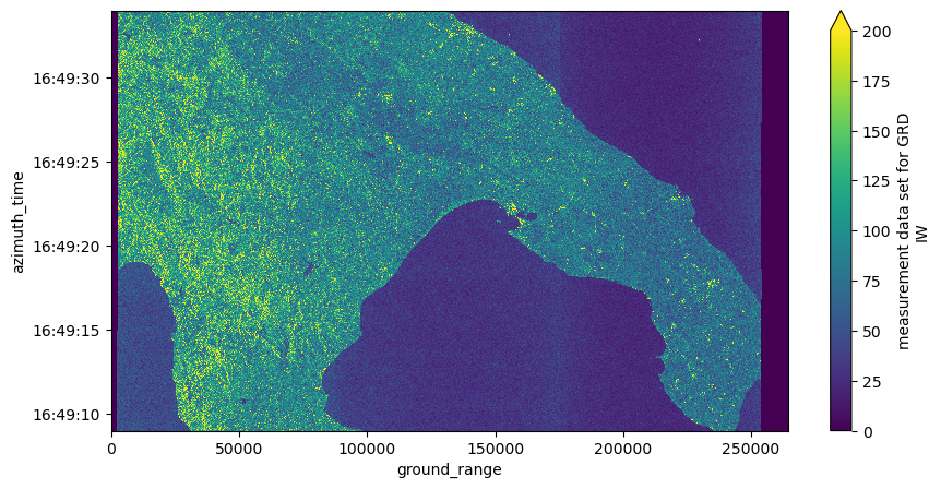

Data Geocoding using GCPs¶

The data we just visualized is in azimuth_time and ground_range coordinates. However, if we would like to create a map or compare this data with other data sources, we need to perform a geocoding (also known as geo-referencing) operation: the data will be interpolated given the reference Ground Control Points (GCPs). GCPs are defined as points on the surface of the Earth of known location used to interpolate and assig new geographic coordinates to the data.
If you want to know more about Sentinel-1 Geocoding, please refer to this geocoding guide specific for GRD data: https://asf.alaska.edu/wp-content/uploads/2019/02/GeocodingSentinelData_GDAL_v7.1_.pdf

Please not that this geocoding process does not involve terrain correction. To match the imagery to actual features on the earth and correct for distortions caused by the side-looking geometry of SAR data, you must perform other steps including terrain correction.

We firstly need to access the GCPs data:

gcp = dt[dt.groups[1]]["conditions/gcp"].to_dataset()
gcp

The GCPs information are provided in a coarser resolution and therefore we need to interpolate them to match the GRD DataArray:

gcp_iterpolated = gcp.interp_like(grd_decimated)
gcp_iterpolated

Assign the interpolated latitude and longitude layers to the GRD coordinates:

grd_decimated = grd_decimated.assign_coords(
    {"latitude": gcp_iterpolated.latitude, "longitude": gcp_iterpolated.longitude}
)

Finally visualize the geocoded data:

_, ax = plt.subplots(subplot_kw={"projection": ccrs.Miller()}, figsize=(12, 8))
gl = ax.gridlines(
    draw_labels=True, crs=ccrs.PlateCarree(), x_inline=False, y_inline=False
)
grd_decimated.plot(
    ax=ax, transform=ccrs.PlateCarree(), x="longitude", y="latitude", vmax=200
)
ax.set_title("Geocoded Sentinel-1 GRD data")
plt.show()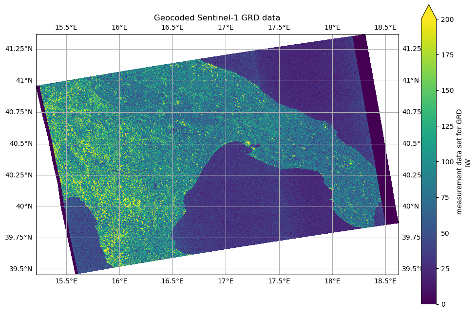

Geographic Selection¶

Now that the data is geocoded/georeferenced, it is possible to perform a spatial slicing (or spatial filtering, or cropping) operation, which allows to select only the data falling in our Area Of Interest (AOI):

lat_max = 40.5
lat_min = 40.25
lon_max = 17
lon_min = 16.5

polygon_lon = [lon_min, lon_max, lon_max, lon_min, lon_min]
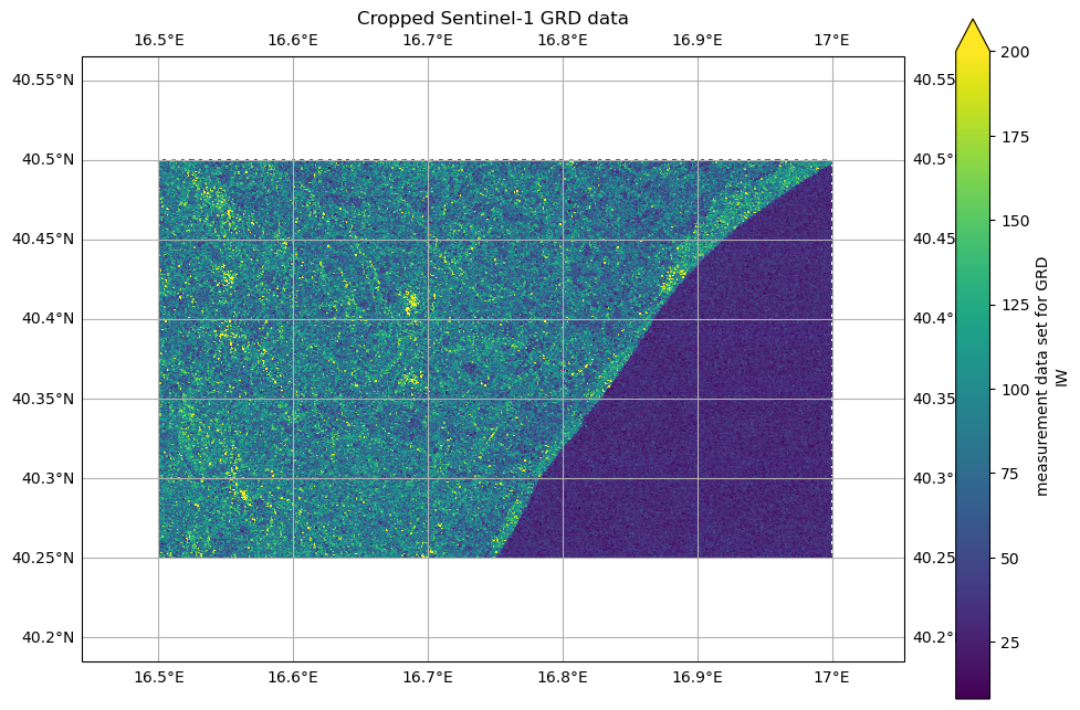
polygon_lat = [lat_max, lat_max, lat_min, lat_min, lat_max]

Crop the data in space, defining a boolean mask and applying it to the data:

mask = (
    (grd_decimated.latitude < lat_max)
    & (grd_decimated.latitude > lat_min)
    & (grd_decimated.longitude < lon_max)
    & (grd_decimated.longitude > lon_min).load().values
)
grd_crop = grd_decimated.where(mask, drop=True)

Plot the result in geographic coordinates, highlighting the Area Of Interest:

_, ax = plt.subplots(subplot_kw={"projection": ccrs.Miller()}, figsize=(12, 8))
gl = ax.gridlines(
    draw_labels=True, crs=ccrs.PlateCarree(), x_inline=False, y_inline=False
)
grd_decimated[::5, ::5].plot(
    ax=ax,
    transform=ccrs.PlateCarree(),
    x="longitude",
    y="latitude",
    vmax=200,
)
plt.plot(
    polygon_lon,
    polygon_lat,
    color="red",
    linewidth=2,
    marker="o",
    transform=ccrs.PlateCarree(),
)
ax.set_title("Geocoded Sentinel-1 GRD data, AOI in red")

_, ax = plt.subplots(subplot_kw={"projection": ccrs.Miller()}, figsize=(12, 8))
gl = ax.gridlines(
    draw_labels=True, crs=ccrs.PlateCarree(), x_inline=False, y_inline=False
)
grd_crop.plot(
    ax=ax,
    transform=ccrs.PlateCarree(),
    x="longitude",
    y="latitude",
    vmax=200,
)
ax.set_title("Cropped Sentinel-1 GRD data")

plt.show()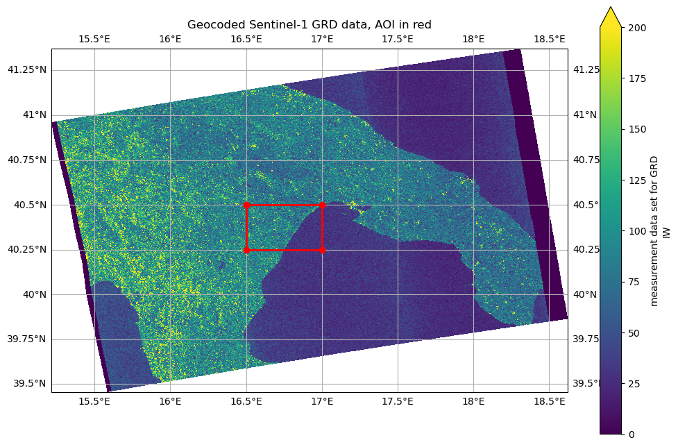

Summary¶

This notebook explored Sentinel-1 GRD data: how to open the Zarr product, select specific groups and perform more advanced operations like geocoding.

Welcome

Introduction to xcube-eopf Data Store.

Welcome

Sentinel-1 L2 OCN Zarr Product Exploration