Sentinel-1 L2 OCN Zarr Product Exploration

Sentinel-1 L2 OCN Zarr Product Exploration¶

Table of Contents¶

Introduction
Import modules
Load and filter the data
Examples of product usage

Introduction¶

In this notebook we will show examples of L2 OCN products and plotting examples with Xarray.

Import Modules¶

import xarray as xr
import matplotlib.pyplot as plt
import numpy as np

Load and filter the data¶

s3_link = "https://objectstore.eodc.eu:2222/e05ab01a9d56408d82ac32d69a5aae2a:sample-data/tutorial_data/cpm_v253/S1A_S5_OCN__2SDV_20230315T185328_20230315T185357_047658_05B968_C2AE.zarr"

datatree = xr.open_datatree(s3_link, engine="zarr")

osw = datatree["osw"]
owi = datatree["owi"]
rvl = datatree["rvl"]

Examples of product usage¶

Ocean Wind Field (OWI)¶

open data

owi = owi["S01SS5OCN_20230315T185328_0029_A272_C2AE_05B968_VV"]

Access the polarisation group or variable within the OWI group

polarisation = owi.conditions["polarisation"]
polarisation

Wind speed¶

_, ax = plt.subplots(nrows=1, ncols=2, figsize=(16, 8))
owi.measurements.wind_speed.plot(ax=ax[0])

polarisation_index = 0
owi.conditions.nrcs[..., polarisation_index].plot(ax=ax[1], vmax=0.04)
ax[0].set_title("Wind speed from copolarised channel")
ax[1].set_title(
    f"NRCS [m^2/m^2] averaged on OWI grid (polarisation: {polarisation.attrs['flag_meanings'].split()[polarisation_index]})"
)
plt.show()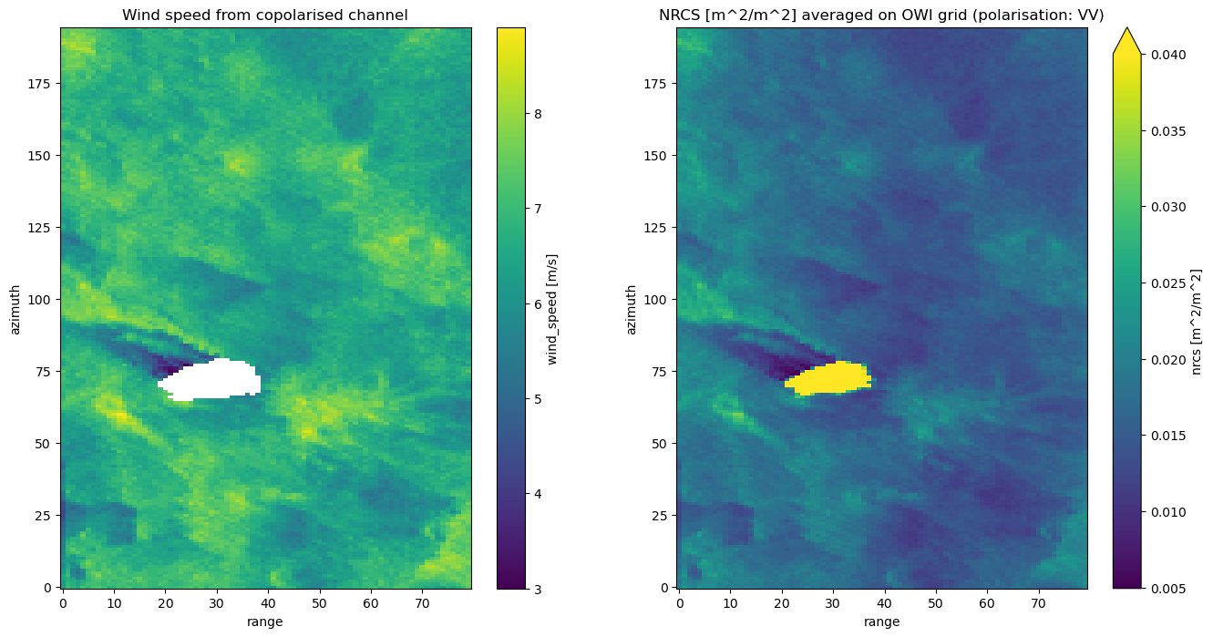

Wind direction¶

Note that in the following plot wind directions are in meteorological convention (directions are measured clockwise from North) without taking into account the platform heading

owi.measurements.wind_direction.plot()
plt.title("Wind direction in meteorological convention")
plt.show()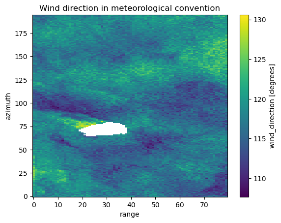

Wind field in geographic projection¶

Vectors can be plotted using the plot.quiver method, but u and y vector components are required as separate variables.

Wind data is provided as a pair of dataarrays:

wind_speed: wind vector module
wind_direction: angle of the wind vector in meteorological convention

The matplotlib.pyplot.quiver method can be used to plot vectors by computing u and v vector components.

x and y point coordinates can optionally be passed as arguments.

Providing lat and lon values projects the data onto geographical coordinates.

Plot

def get_vector_uv(norm, direction, heading=0):
    direction = (
        direction - heading
    )  # conversion from wind direction wrt north to wind direction wrt azimuth
    direction += 180.0  # conversion from meteorological to oceanographic conventions ("from where the wind comes" to "to where the wind goes")
    direction = (
        90 - direction
    )  # conversion from (z-axis, clockwise) angle to cartesian convention (x-axis, anti-clockwise))
    u = norm * np.cos(np.deg2rad(direction))
    v = norm * np.sin(np.deg2rad(direction))
    return u, v


stride = 5
wind_speed = owi.measurements.wind_speed[
    ::stride, ::stride
]  # also as the arrow color criterion
wind_dir = owi.measurements.wind_direction[::stride, ::stride]
u, v = get_vector_uv(wind_speed, wind_dir)
cp = plt.contourf(
    owi.measurements.longitude,
    owi.measurements.latitude,
    owi.measurements.wind_speed,
    cmap="jet",
)
plt.quiver(
    owi.measurements.longitude[::stride, ::stride],
    owi.measurements.latitude[::stride, ::stride],
    u,
    v,
    wind_speed,
)
cbar = plt.colorbar(cp)
cbar.ax.set_ylabel(
    owi.measurements.wind_speed._eopf_attrs["long_name"]
    + f" [{owi.measurements.wind_speed._eopf_attrs['units']}]"
)
plt.xlabel(owi.measurements.longitude.attrs["long_name"])
plt.ylabel(owi.measurements.latitude.attrs["long_name"])
plt.title("Wind Field")
plt.show()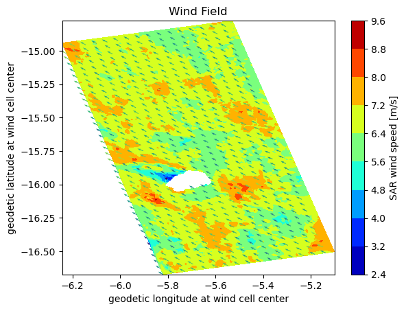

Ocean Swell Wave (OSW)¶

osw = osw["S01SS5OCN_20230315T185328_0029_A272_C2AE_05B968_VV"]
osw

Normalized Radar Cross Section (NRCS) averaged on OSW grid¶

osw.conditions.nrcs.plot()
plt.title("NRCS [dB] averaged on OSW grid")
plt.show()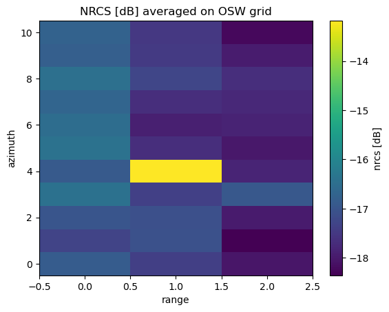

Significant wave height¶

partition_index = 0
osw.measurements.hs[..., partition_index].plot()
plt.title(f"Significant Wave Height [m] (partition: {partition_index})")
plt.show()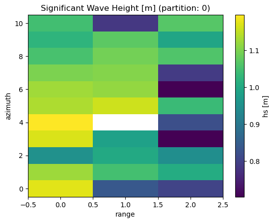

Dominant Wave Length¶

partition_index = 0
osw.measurements.wave_length[..., partition_index].plot()
plt.title(f"Dominant Wave Length [m] (partition: {partition_index})")
plt.show()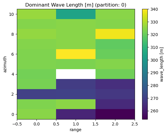

Swell wave field in geographic projection¶

partition_index = 0
wave_direction = osw.measurements.wave_direction[..., partition_index]
wave_height = osw.measurements.hs[..., partition_index]
u, v = get_vector_uv(wave_height, wave_direction)
cp = plt.contourf(
    osw.measurements.longitude, osw.measurements.latitude, wave_height, cmap="jet"
)
cbar = plt.colorbar(cp)

plt.quiver(osw.measurements.longitude, osw.measurements.latitude, u, v, cmap="jet")
cbar.ax.set_ylabel(
    osw.measurements.hs._eopf_attrs["long_name"]
    + f" [{osw.measurements.hs.attrs['units']}]"
)
plt.xlabel(osw.measurements.longitude.attrs["long_name"])
plt.ylabel(osw.measurements.latitude.attrs["long_name"])
plt.title(f"Swell Wave Field (partition: {partition_index})")
plt.show()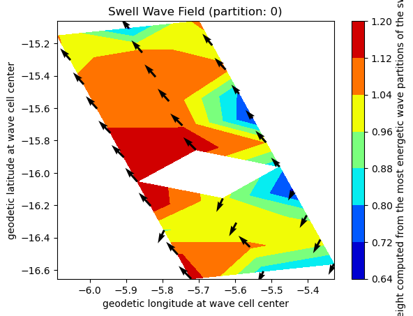

Swell Spectrum in polar coordinates¶

cell_index = 10, 2
osw.conditions.polar_spectrum[cell_index].plot()
plt.title(f"Swell Spectrum in Polar Coordinates (cell: {list(cell_index)})")
plt.show()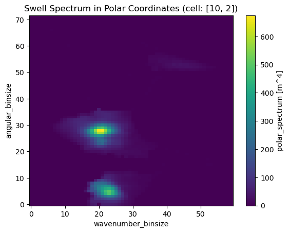

Ocean Radial Velocity (RVL)¶

rvl = datatree["rvl"]
rvl = rvl["S01SS5OCN_20230315T185328_0029_A272_C2AE_05B968_VV"]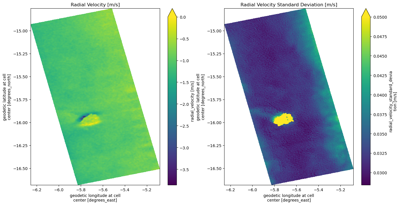
rvl

Radial velocity in geographic projection¶

_, ax = plt.subplots(nrows=1, ncols=2, figsize=(16, 8))
rvl.measurements.radial_velocity.plot(x="longitude", y="latitude", vmax=0, ax=ax[0])
rvl.measurements.radial_velocity_standard_deviation.plot(
    x="longitude", y="latitude", ax=ax[1], vmax=0.05
)
ax[0].set_title("Radial Velocity [m/s]")
ax[1].set_title("Radial Velocity Standard Deviation [m/s]")
plt.show()

Welcome

Sentinel-1 GRD Zarr Product Exploration

Welcome

SENTINEL-1 L1 SLC TOPSAR Product Format Prototype