SENTINEL-1 L1 SLC TOPSAR Product Format Prototype

Table of Contents¶

Introduction
Import modules
File path definition
Read local files with EOPF
Read remote files with xarray-datatree
Examples of product usage
A. Orbit interpolation
B. Calibration
C. Geocoding using GCPs
D. RGB Plot of two non coregistred burst

Introduction¶

In this notebook we will show an example of slc TOPSAR product and some easy usage examples

Objectives:

Allow easy access to the bursts, since they are the data unit that is typically processed
Provide ready-to-use datasets and data variable
Allow users to open and manipulate data using both standard external tools and the EOPF

Relevant Features:

Swaths, bursts and polarization are separeted in different products
The coordinates associated to the data are the physical coordinates
The zarr product will adhere to CF convetion (this will allow the user to open the prodoct with standards tools, such as xarray, exploiting properly the data coordinates).
STAC attributes(Will be added in future)

Notes:

It is a preliminary example of product

Not all the metadata are included in these product prototype, but they will be included in the future.
Among the excluded metadata, there are:
- RFI
- qualityInformation
- downlinkInformation
The stac attrabutes are still to be defined.
The name of the variables are preliminary and they may change in the future.
Variable attributes will be refined in the future, including:
- long_name
- units
- and standard names for coordinates
The chunking is not defined yet.
Products naming convention is to be defined.
Reading from local and remote storage with EOPF is experimental(branch feat/coords_in_vars, commit 10a4f2e1) and not offically released.

Import modules¶

Dependencies

datatree
eopf
xarray
matplotlib
cartopy
fsspec

%matplotlib inline

import datatree
import numpy as np
import xarray as xr

import matplotlib.pyplot as plt

plt.rcParams["figure.figsize"] = (10, 5)
plt.rcParams["font.size"] = 10

File path definition¶

Product Defnition¶

swath = "IW1"
polarization = "VH"
burst_id = "249411"

zarr_name_1 = "S01SIWSLC_20231201T170634_0067_A117_S000_5464A_VH_IW1_249411"
zarr_name_2 = "S01SIWSLC_20231119T170635_0067_A117_S000_5464A_VH_IW1_249411"

Remote files path

remote_product_path_1 = f"https://storage.sbg.cloud.ovh.net/v1/AUTH_8471d76cdd494d98a078f28b195dace4/sentinel-1-public/demo_product/slc/{zarr_name_1}.zarr/"
remote_product_path_2 = f"https://storage.sbg.cloud.ovh.net/v1/AUTH_8471d76cdd494d98a078f28b195dace4/sentinel-1-public/demo_product/slc/{zarr_name_2}.zarr/"

Local files

The listed files do not work with the latest eopf-cpm library and therefore the next cells are commented out

# # Download the files into the folder ./scratch/demo_product/slc/
# !wget -q -r -nc -nH --cut-dirs=5 https://storage.sbg.cloud.ovh.net/v1/AUTH_8471d76cdd494d98a078f28b195dace4/sentinel-1-public/demo_product/slc --no-parent -P ./scratch/demo_product/slc/ --reject "index.html*"

# # Set the local product paths using the specified directory
# local_product_path_1 = f"./scratch/demo_product/slc/{zarr_name_1}.zarr/"
# local_product_path_2 = f"./scratch/demo_product/slc/{zarr_name_2}.zarr/"

Read local files with EOPF¶

# store = EOZarrStore(local_product_path_1)
# store = store.open()
# store

# store.load()

Read remote files with xarray-datatree¶

(xarray extension that allow performing operations on hierachical structures)

dt = datatree.open_datatree(remote_product_path_1, engine="zarr", chunks={})
dt

Examples of product usage¶

Orbit interpolation¶

open data

burst = xr.open_dataset(remote_product_path_1, group="measurements", engine="zarr")[
    "slc"
]
orbit = xr.open_dataset(remote_product_path_1, group="conditions/orbit", engine="zarr")

orbit.plot.scatter(y="azimuth_time", x="position", hue="velocity", cmap="Blues")
plt.show()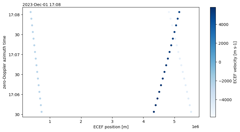

Interpolate

interp_orbit = orbit.interp_like(burst.azimuth_time)

Plot

orbit.plot.scatter(y="azimuth_time", x="position", hue="velocity", cmap="Blues")
interp_orbit.plot.scatter(y="azimuth_time", x="position", color="red")
plt.show()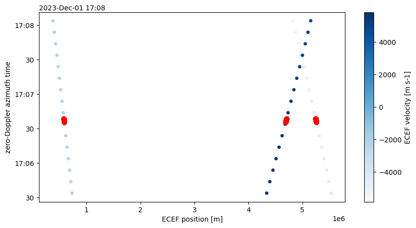

Calibration¶

Open Calibration lut data

calibration_lut = xr.open_dataset(
    remote_product_path_1, group="quality/calibration", engine="zarr"
)

Calibrate Data

calibration_matrix = calibration_lut.interp_like(burst)
calibrated_measurement = burst / calibration_matrix["sigma_nought"]

Plot Full Data

plt.figure(figsize=(20, 4))
_ = abs(burst).plot(y="azimuth_time", vmax=200)

Geocoding using GCPs¶

Open GCP Data

gcp = xr.open_dataset(remote_product_path_1, group="conditions/gcp", engine="zarr")

Interpolate and assign new geographic coordinates

gcp_iterpolated = gcp.interp_like(burst)
burst = burst.assign_coords(
    {"latitude": gcp_iterpolated.latitude, "longitude": gcp_iterpolated.longitude}
)

Plot Subset

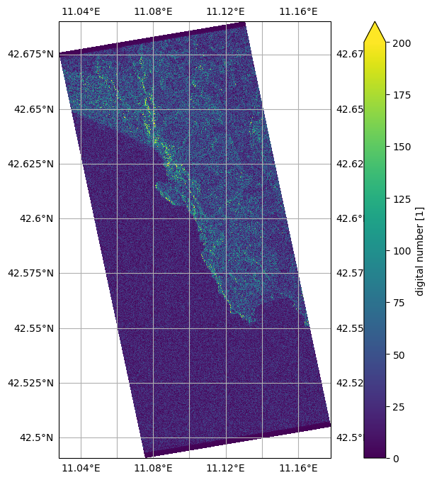
import cartopy.crs as ccrs

_, ax = plt.subplots(subplot_kw={"projection": ccrs.Miller()}, figsize=(12, 8))
gl = ax.gridlines(
    draw_labels=True, crs=ccrs.PlateCarree(), x_inline=False, y_inline=False
)
abs(burst[:, 7000:9000]).plot(
    ax=ax, transform=ccrs.PlateCarree(), x="longitude", y="latitude", vmax=200
)
plt.show()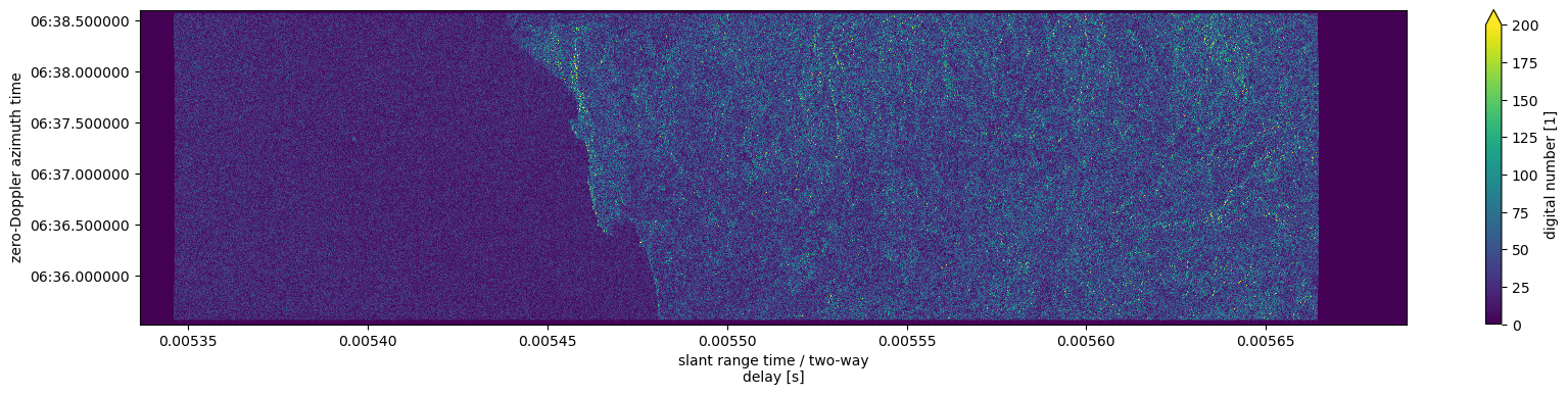

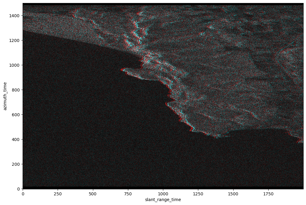
RGB Plot of two non coregistred burst¶

The RBG plot shows the shift between the non coregistred bursts

swath:IW1
polarization:VH
burst_id:249411
burst acquisition date:
- 2023-12-01
- 2023-11-19

Open Data

slc_1 = xr.open_dataset(remote_product_path_1, group="measurements", engine="zarr")[
    "slc"
]
slc_2 = xr.open_dataset(remote_product_path_2, group="measurements", engine="zarr")[
    "slc"
]

amp_1 = np.abs(slc_1).drop_vars(["azimuth_time", "slant_range_time"])
amp_2 = np.abs(slc_2).drop_vars(["azimuth_time", "slant_range_time"])

Compose RGB

rgb = xr.concat([amp_1, amp_2, amp_2], dim="rgb")
rgb = xr.where(rgb > 200, 200, rgb) / 200

Plot Subset

plt.figure(figsize=(12, 8))
rgb[:, :, 7000:9000].plot.imshow(rgb="rgb")
plt.show()

Welcome

Sentinel-1 L2 OCN Zarr Product Exploration

Welcome

Sentinel-3 Patchwork L1 OLCI EFR L2 SLSTR FPR SYN AOD product format prototype