Introduction to xarray-eopf backend.

Table of Contents¶

Introduction
Install the xarray-eopf Backend
Import modules
Main Features of the xarray-eopf Backend
Open the Product in Native Mode
Open the Product in Analysis Mode
Integration with the STAC Item
Conclusion

Introduction¶

xarray-eopf is a Python package that extends xarray with a custom backend called "eopf-zarr". This backend enables seamless access to ESA EOPF data products stored in the Zarr format, presenting them as analysis-ready data structures.

This notebook demonstrates how to use the xarray-eopf backend to explore and analyze EOPF Zarr datasets. It highlights the key features currently supported by the backend.

🐙 GitHub: EOPF Sample Service – xarray-eopf
❗ Issue Tracker: Submit or view issues
📘 Documentation: xarray-eopf Docs

Install the xarray-eopf Backend¶

The backend is implemented as an xarray plugin and can be installed using either pip or conda/mamba from the conda-forge channel.

📦 PyPI: xarray-eopf on PyPI pip install xarray-eopf
🐍 Conda (conda-forge): xarray-eopf on Anaconda conda install -c conda-forge xarray-eopf
You can also use Mamba as a faster alternative to Conda: mamba install -c conda-forge xarray-eopf

Import Modules¶

The xarray-eopf backend is implemented as a plugin for xarray. Once installed, it registers automatically and requires no additional import. You can simply import xarray as usual:

import matplotlib.colors as mcolors
import matplotlib.pyplot as plt
import numpy as np
import pystac_client
import xarray as xr

xr.set_options(display_expand_attrs=False)

<xarray.core.options.set_options at 0x7a08726c7b60>

Main Features of the xarray-eopf Backend¶

The xarray-eopf backend for EOPF data products can be selecterd by setting engine="eopf-zarr" in xarray.open_dataset(..) and xarray.open_datatree(..) method. It supports two modes of operation:

Analysis Mode (default)
Native Mode

Native Mode¶

Represents EOPF products without modification using xarray’s DataTree and Dataset.

open_dataset(..) — Returns a flattened version of the data tree
open_datatree(..) — Returns the full DataTree, same as xr.open_datatree(.., engine="zarr")

Analysis Mode¶

Provides an analysis-ready, resampled view of the data (currently for Sentinel-2 only).

open_dataset(..) — Loads Sentinel-2 products in a harmonized, analysis-ready format
open_datatree(..) — Not implemented in this mode (NotImplementedError)

📚 More info: xarray-eopf Guide

Open the Product in Native Mode¶

Sentinel-2 Level-2A¶

We begin with a simple example by accessing a Sentinel-2 L2A product in native mode. To obtain the product URL, you can use the STAC Browser to locate a tile and retrieve the URL from the “EOPF Product” asset.

path = (
    "https://objectstore.eodc.eu:2222/e05ab01a9d56408d82ac32d69a5aae2a:202505-s02msil2a/18/products"
    "/cpm_v256/S2B_MSIL2A_20250518T112119_N0511_R037_T29RLL_20250518T140519.zarr"
)

As explained above, we can use xr.open_datatree to open the EOPF Zarr product as an xr.DataTree. Note that you still need to include the argument chunks={} — this is required by a wrapper function in xarray after the data is opened by the backend implementation.

dt = xr.open_datatree(path, engine="eopf-zarr", op_mode="native", chunks={})
dt

As an example, we plot the quicklook image to view the RGB image.

dt.quality.l2a_quicklook.r60m.tci

dt.quality.l2a_quicklook.r60m.tci.plot.imshow(rgb="band")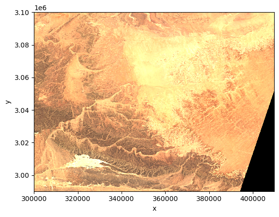

The xarray.DataTree data model is relatively new, introduced in xarray v2024.10.0 (October 2024). To support compatibility with existing workflows that rely on the traditional xr.Dataset model, we provide the function xarray.open_dataset(path, engine="eopf-zarr", op_mode="native", **kwargs). This function flattens the DataTree structure and returns a single xr.Dataset.

In this process, hierarchical groups within the Zarr product are removed by converting their contents into standalone datasets and merging them into one. To ensure uniqueness, variable and dimension names are prefixed with their original group paths, using an underscore (_) as the default separator. For example, a variable named b02 located in the group measurements/reflectance/r10m will be renamed to measurements_reflectance_r10m_b02 in the returned dataset.

ds = xr.open_dataset(path, engine="eopf-zarr", op_mode="native", chunks={})
ds

The separator character used in flattened variable names can be customized via the group_sep parameter. Additionally, you can filter the returned variables using the variables keyword argument, which accepts a string, an iterable of names, or a regular expression (regex) pattern.

ds = xr.open_dataset(
    path,
    engine="eopf-zarr",
    op_mode="native",
    chunks={},
    group_sep="/",
    variables="quality/l2a_quicklook/r60m/*",
)
ds

Following the previous steps, we can now select a data variable and display the quicklook RGB image as an example.

ds["quality/l2a_quicklook/r60m/tci"].plot.imshow(rgb="quality/l2a_quicklook/r60m/band")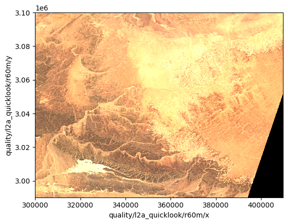

Sentinel-1 GRD¶

Lets show a second example where we want to open a Sentinel-1 GRD product with the "eopf-zarr" engine.

path = (
    "https://objectstore.eodc.eu:2222/e05ab01a9d56408d82ac32d69a5aae2a:sample-data/tutorial_data/"
    "cpm_b716/S1A_IW_GRDH_1SDV_20170508T164830_20170508T164855_016493_01B54C_8604.zarr"
)

First, we use xr.open_datatree to open the EOPF Zarr product as an xr.DataTree.

dt = xr.open_datatree(path, engine="eopf-zarr", op_mode="native", chunks={})
dt

Similarly, we can open the Sentinel-1 GRD Zarr product using xr.open_dataset to obtain an xr.Dataset, just as we did earlier for the Sentinel-2 L2A product, where we filter by "VH_measurements*".

ds = xr.open_dataset(
    path, engine="eopf-zarr", op_mode="native", chunks={}, variables="VH_measurements*"
)
ds

As a final step, we plot the VH measurement to provide a visual example of the data.

ds["VH_measurements_grd"][::10, ::10].plot(vmax=200)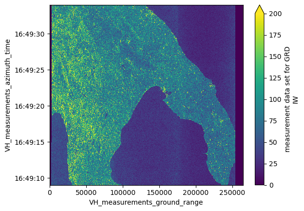

Open the Product in Analysis Mode¶

Currently, analysis mode is available only for Sentinel-2 products. Support for Sentinel-3 and Sentinel-1 will be added in upcoming releases.

The analysis mode is designed to present EOPF data products in an analysis-ready and user-friendly format using xarray’s Dataset data model. For Sentinel-2 products, it applies a unified grid mapping across all data variables, meaning selected variables are spatially upscaled or downscaled as needed. This ensures the resulting dataset uses a single, consistent pair of x and y coordinates for all variables.

Native resolution of each Sentinel-2 spectral band¶

10m: [b02, b03, b04, b08]
20m: [b05, b06, b07, b8a, b11, b12]
60m: [b01, b09, b10]

Analysis mode for Sentinel-2¶

The analysis mode for Sentinel-2 has the following key properties:

Default mode when using the "eopf-zarr" backend.
Spatial resolution options: Users can choose between 10m, 20m, and 60m, with 10m as the default.
Upsampling:
- Performed via 2D interpolation controlled by the spline_orders argument.
- Accepts a single spline order for all variables or a dictionary mapping spline orders to variable names or data types.
- Supported spline orders: 0 (nearest neighbor, default for scl), 1 (linear), 2 (bi-linear), 3 (cubic, default).
Downsampling:
- Done through aggregation methods governed by the agg_methods argument.
- Can be a single method for all variables or a dictionary mapping methods to variable names or data types.
- Available methods include "center" (default for scl), "count", "first", "last", "max", "mean" (default), "median", "mode", "min", "prod", "std", "sum", and "var".
Variable selection: Specific variables can be selected via the variables argument, which accepts a variable name, a regex pattern, or an iterable of either.

More details are available in the documentation.

Note: Default up- and downsampling methods follow ESA’s Sentinel-2 Level 2A guidelines (documentation PDF).

path = (
    "https://objectstore.eodc.eu:2222/e05ab01a9d56408d82ac32d69a5aae2a:202505-s02msil2a/18/products"
    "/cpm_v256/S2B_MSIL2A_20250518T112119_N0511_R037_T29RLL_20250518T140519.zarr"
)

By default, without specifying any keyword arguments, the function returns an xr.Dataset with all spectral bands at 10m spatial resolution.

%%time
ds_default = xr.open_dataset(path, engine="eopf-zarr", chunks={})
ds_default

Now, we can explore how to configure the processing using the available keyword arguments.

ds_nearest = xr.open_dataset(
    path,
    engine="eopf-zarr",
    chunks={},
    spline_orders=0,
    variables=["b01", "b02", "scl"],
)
ds_nearest

We can now compare the different upsampling methods for “b01”, which native resolution is at 60m.

fig, ax = plt.subplots(1, 3, figsize=(18, 5))
ds_default.b01[:1000, :1000].plot(ax=ax[0], vmin=0.0, vmax=0.2)
ax[0].set_title("Cubic interpolation")
ds_nearest.b01[:1000, :1000].plot(ax=ax[1], vmin=0.0, vmax=0.2)
ax[1].set_title("Nearest neighbor interpolation")
(ds_default.b01 - ds_nearest.b01)[:1000, :1000].plot(
    ax=ax[2], vmin=-0.01, vmax=0.01, cmap="bwr"
)
ax[2].set_title("Difference")
plt.tight_layout()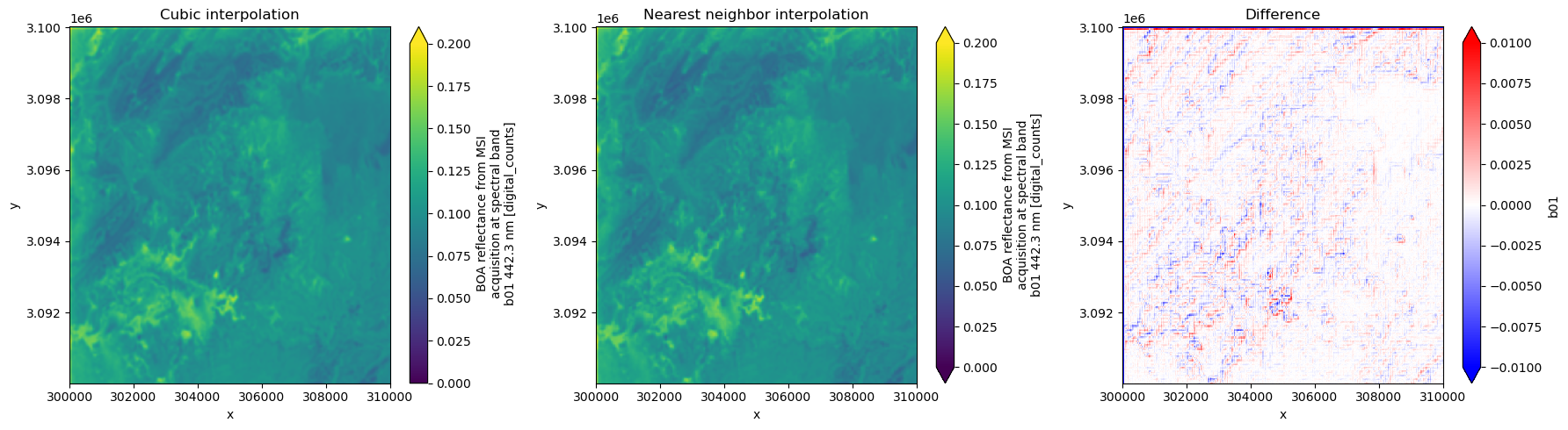

Scene classification layer in Sentinel-2 L2A product¶

For the SCL, the flag names, values, and corresponding colors are added to the attributes to facilitate plotting. The colors are defined according to Sentinel Hub’s specifications.

path = (
    "https://objectstore.eodc.eu:2222/e05ab01a9d56408d82ac32d69a5aae2a:202504-s02msil2a/30/"
    "products/cpm_v256/S2B_MSIL2A_20250430T101559_N0511_R065_T32TLQ_20250430T131328.zarr"
)

ds = xr.open_dataset(path, engine="eopf-zarr", chunks={}, resolution=60)
ds

fig, ax = plt.subplots(1, 2, figsize=(12, 5))

ds.b04.plot(ax=ax[0], vmin=0.0, vmax=0.3)
ax[0].set_title("B04 - red")

cmap = mcolors.ListedColormap(ds.scl.attrs["flag_colors"].split(" "))
nb_colors = len(ds.scl.attrs["flag_values"])
norm = mcolors.BoundaryNorm(
    boundaries=np.arange(nb_colors + 1) - 0.5, ncolors=nb_colors
)
im = ds.scl.plot.imshow(ax=ax[1], cmap=cmap, norm=norm, add_colorbar=False)
cbar = fig.colorbar(im, ax=ax[1], ticks=ds.scl.attrs["flag_values"])
cbar.ax.set_yticklabels(ds.scl.attrs["flag_meanings"].split(" "))
cbar.set_label("Class")
ax[1].set_title("Scene classification layer")

plt.tight_layout()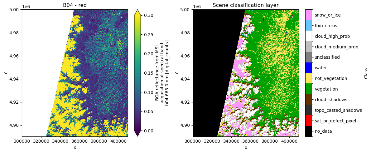

Sentinel-2 L1C¶

Let’s now open a Sentinel-2 L1C product. In this product, each band is available only at its native resolution. This allows us to demonstrate the aggregation mode used during downsampling.

path = (
    "https://objectstore.eodc.eu:2222/e05ab01a9d56408d82ac32d69a5aae2a:202504-s02msil1c/30/products"
    "/cpm_v256/S2B_MSIL1C_20250430T101559_N0511_R065_T32TLQ_20250430T124542.zarr"
)

As explained above, the default aggregation method for spectral bands during downsampling is to take the mean of the superpixel.

ds_agg_mean = xr.open_dataset(path, engine="eopf-zarr", chunks={}, resolution=60)
ds_agg_mean

As a second dataset, we apply "max" as aggregation mode.

ds_agg_max = xr.open_dataset(
    path, engine="eopf-zarr", chunks={}, resolution=60, agg_methods="max"
)
ds_agg_max

Next, we plot the spectral band B04 (red) alongside the difference between the two aggregation modes.

fig, ax = plt.subplots(1, 3, figsize=(18, 5))
ds_agg_max.b04[1000::, 1000::].plot(ax=ax[0], vmin=0.0, vmax=0.2)
ax[0].set_title("Aggregation method 'max'")
ds_agg_mean.b04[1000::, 1000::].plot(ax=ax[1], vmin=0.0, vmax=0.2)
ax[1].set_title("Aggregation method 'mean'")
(ds_agg_max.b04 - ds_agg_mean.b04)[1000::, 1000::].plot(
    ax=ax[2], vmin=-0.05, vmax=0.05, cmap="bwr"
)
ax[2].set_title("Difference")
plt.tight_layout()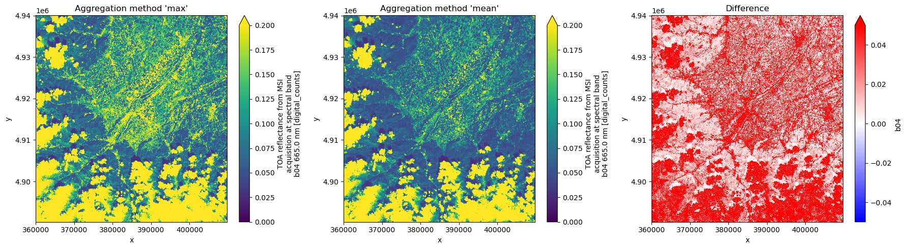

Integration with the STAC Item¶

The STAC API at https://stac.core.eopf.eodc.eu allows searching for tiles by bounding box and time range.
The "product" asset can be used to open an EOPF Zarr product.
Additional fields in the asset provide the parameters required to open the dataset.
Assets representing individual bands are also available; xarray integration for these is still a work in progress.

First, we use pystac_client to query the catalog based on a given bounding box and temporal range.

catalog = pystac_client.Client.open("https://stac.core.eopf.eodc.eu")
items = list(
    catalog.search(
        collections=["sentinel-2-l2a"],
        bbox=[7.2, 44.5, 7.4, 44.7],
        datetime=["2025-04-30", "2025-05-01"],
    ).items()
)
items

[<Item id=S2B_MSIL2A_20250430T101559_N0511_R065_T32TLQ_20250430T131328>]

Next, we can inspect the item’s contents, including the additional field xarray:open_datatree_kwargs, which provides the arguments needed to open the product using xarray’s eopf-zarr engine.

item = items[0]
item.assets["product"]

We can now use the href and xarray:open_datatree_kwargs from the item to open the product.

ds = xr.open_datatree(
    item.assets["product"].href,
    **item.assets["product"].extra_fields["xarray:open_datatree_kwargs"]
)
ds

The same applies to the xr.open_dataset method, which returns a flattened DataTree represented as an xr.Dataset.

ds = xr.open_dataset(
    item.assets["product"].href,
    **item.assets["product"].extra_fields["xarray:open_datatree_kwargs"]
)
ds

Conclusion¶

This notebook presents the current development state of the xarray-eopf backend, which enables seamless access to EOPF Zarr products using familiar xarray methods such as xr.open_dataset and xr.open_datatree by specifying engine="eopf-zarr". The key takeaways are summarized below:

Two operation modes are available:
- op_mode="native":
  Represents EOPF products without modification using xarray’s DataTree and Dataset structures.
  Example: xr.open_dataset(path, engine="eopf-zarr", op_mode="native") returns the data tree as a flattened xr.Dataset.
- op_mode="analysis":
  Provides an analysis-ready, resampled view of the data (currently supported for Sentinel-2 only). Features include:
  - Up- or downsampling Sentinel-2 bands to a common user-defined spatial resolution.
  - Enhanced metadata for the Sentinel-2 Level 2A scene classification layer, enabling standardized visualization.
Opening parameters are fully integrated into the STAC items, facilitating streamlined data access and management.

Future Development Steps¶

Extend analysis mode support to Sentinel-1 and Sentinel-3 data.
Incorporate user feedback—please test the plugin and submit issues here: https://github.com/EOPF-Sample-Service/xarray-eopf/issues
Continue active development of the plugin through November 2024 (at least within the EOPF Sample Zarr Service project).

Jupyter Notebooks

NDVI-based approach to study Landslide areas

Jupyter Notebooks

SENTINEL-1 L1 GRD Product Format Prototype