Parcel delineation using Sentinel-2
Delineating agricultural parcels based on a neural network, using Sentinel-2 input data

Table of contents
Run this notebook interactively with all dependencies pre-installed
Preface
The original notebook used as a starting point for this work is a Copernicus Data Space Ecosystem example, available here, originally created by VITO (see the CDSE notebook for the original authors).
The example has been adapted to use the data provided by the EOPF Zarr Samples project instead of the openEO API.
Introduction
In this notebook we will be performing parcel delineation using Sentinel-2 Zarr data. The process involves reading the Sentinel-2 data, calculating the NDVI (Normalized Difference Vegetation Index), and applying a pre-trained neural network model to segment the parcels.
Setup
Start importing the necessary libraries
import os
from datetime import datetime

import matplotlib.pyplot as plt
import s3fs
import xarray as xr
from distributed import LocalCluster
from pyproj import Transformer

from parcel_delineation_utils import apply_filter, apply_segmentation_parallel
cluster = LocalCluster(processes=False)
client = cluster.get_client()
cluster/home/mclaus@eurac.edu/micromamba/envs/eopf-zarr3/lib/python3.11/site-packages/distributed/node.py:187: UserWarning: Port 8787 is already in use.
Perhaps you already have a cluster running?
Hosting the HTTP server on port 38615 instead
warnings.warn(
Find required data
bucket = "e05ab01a9d56408d82ac32d69a5aae2a:sample-data"
prefix = "tutorial_data/cpm_v253/"
prefix_url = "https://objects.eodc.eu"
# Create the S3FileSystem with a custom endpoint
fs = s3fs.S3FileSystem(anon=True, client_kwargs={"endpoint_url": prefix_url})

# unregister handler to make boto3 work with CEPH
handlers = fs.s3.meta.events._emitter._handlers
handlers_to_unregister = handlers.prefix_search("before-parameter-build.s3")
handler_to_unregister = handlers_to_unregister[0]
fs.s3.meta.events._emitter.unregister(
    "before-parameter-build.s3", handler_to_unregister
)

s3path = "s3://" + f"{bucket}/{prefix}" + "S2*_MSIL2A_*_*_*_T31UFS_*.zarr"
remote_files = fs.glob(s3path)
paths = [f"{prefix_url}/{f}" for f in remote_files]

print(len(paths))
12
Read EOPF Zarr
In this step, we read the Zarr data and perform spatial filtering. Then we open the 10 meter band data as well as the SCL, which we will use for cloud masking.
ds = xr.open_datatree(paths[0], engine="zarr", chunks={}, decode_timedelta=False)
target_crs = ds.attrs["stac_discovery"]["properties"]["proj:epsg"]
print(f"Target CRS of the selected Sentinel-2 tiles: {target_crs}")

spatial_extent = {
    "west": 5.0,
    "south": 51.2,
    "east": 5.1,
    "north": 51.3,
}
transformer = Transformer.from_crs("EPSG:4326", "EPSG:32631", always_xy=True)
west_utm, south_utm = transformer.transform(
    spatial_extent["west"], spatial_extent["south"]
)
east_utm, north_utm = transformer.transform(
    spatial_extent["east"], spatial_extent["north"]
)

x_slice = slice(west_utm, east_utm)
y_slice = slice(north_utm, south_utm)


def extract_time_and_crop(ds):
    date_format = "%Y%m%dT%H%M%S"
    filename = ds.encoding["source"]
    date_str = os.path.basename(filename).split("_")[2]
    time = datetime.strptime(date_str, date_format)
    ds = ds.assign_coords(time=time)
    return ds.sel(x=x_slice, y=y_slice)
Target CRS of the selected Sentinel-2 tiles: 32631
r10m = xr.open_mfdataset(
    paths,
    engine="zarr",
    chunks={},
    group="/measurements/reflectance/r10m",
    concat_dim="time",
    combine="nested",
    preprocess=extract_time_and_crop,
    decode_cf=False,
    mask_and_scale=False,
)

scl = xr.open_mfdataset(
    paths,
    engine="zarr",
    chunks={},
    group="conditions/mask/l2a_classification/r20m",
    concat_dim="time",
    combine="nested",
    preprocess=extract_time_and_crop,
    decode_cf=False,
    mask_and_scale=False,
)

r10m.rio.write_crs(target_crs, inplace=True)
r10m = r10m.sortby("time")

scl.rio.write_crs(target_crs, inplace=True)
scl = scl.sortby("time")

r10mSelect, validate, and apply mask
Here we prepare and interpolate the mask to align with the 10 meters bands, so that we can apply it over the data.
def validate_scl(scl):
    invalid = [0, 1, 3, 7, 8, 9, 10]  # NO_DATA, SATURATED, CLOUD, etc.
    return ~scl.isin(invalid)


mask_scl_r10m = scl.scl.chunk(chunks={"x": -1, "y": -1}).interp(
    x=r10m["x"], y=r10m["y"], method="nearest"
)

valid_mask = validate_scl(mask_scl_r10m)
masked = r10m.where(valid_mask)
maskedCalculate NDVI
In this step, we calculate NDVI using the masked data as input. The resulting NDVI will be used for running the inference.
We also save the NDVI data to a local Zarr, as this makes it more efficient when running the inference.
def calculate_ndvi(ds: xr.Dataset) -> xr.DataArray:
    """Calculate NDVI from dataset with B04 and B08"""
    red = (ds["b04"] * ds["b04"].attrs["_eopf_attrs"]["scale_factor"]) + ds[
        "b04"
    ].attrs["_eopf_attrs"]["add_offset"]

    nir = (ds["b08"] * ds["b08"].attrs["_eopf_attrs"]["scale_factor"]) + ds[
        "b08"
    ].attrs["_eopf_attrs"]["add_offset"]

    return (nir - red) / (nir + red)


ndvi = calculate_ndvi(masked)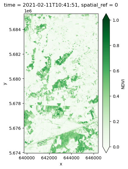
ndviVisualize a sample date for NDVI
ndvi.isel(time=1).plot.imshow(
    cmap="Greens",
    vmin=0,
    vmax=1,
    aspect=0.66,
    size=6,
    add_colorbar=True,
    cbar_kwargs={"label": "NDVI"},
)
# Save the NDVI to Zarr to speed up inference
ndvi_rechunked = ndvi.chunk({"time": 4, "y": 400, "x": 667})

ndvi_rechunked.name = "NDVI"
ndvi_rechunked = ndvi_rechunked.to_dataset()

ndvi_rechunked.to_zarr("ndvi.zarr", mode="w", consolidated=True)
<xarray.backends.zarr.ZarrStore at 0x7fd23dce6520>Download neural networks
Here we download and the pretrained neural networks used for parcel delineation. The networks are downloaded to a local directory, so that we can use them for inference.
models_url = "https://artifactory.vgt.vito.be:443/artifactory/auxdata-public/openeo/parcelDelination/BelgiumCropMap_unet_3BandsGenerator_Models.zip"

os.system(f"wget {models_url} -O models.zip")
os.system("unzip -o models.zip -d onnx_models")
os.system("rm models.zip")Archive: models.zip
inflating: onnx_models/BelgiumCropMap_unet_3BandsGenerator_Network1.onnx
inflating: onnx_models/BelgiumCropMap_unet_3BandsGenerator_Network2.onnx
inflating: onnx_models/BelgiumCropMap_unet_3BandsGenerator_Network3.onnx
0Run segmentation over NDVI
In the parcel_delineation_utils.py file, we have prepared the code that needs to be run for the inference. We simply open the NDVI data, and apply the neural networks to it.
After running the inference, we need to transpose the data, so that it is oriented correctly.
ndvi = xr.open_zarr("ndvi.zarr", consolidated=True)
ndvi = ndvi["NDVI"]
# Run the segmentation model
result = apply_segmentation_parallel(ndvi)
2025-08-20 13:57:41.300013588 [W:onnxruntime:Default, upsamplebase.h:178 UpsampleBase] `tf_half_pixel_for_nn` is deprecated since opset 13, yet this opset 13 model uses the deprecated attribute
2025-08-20 13:57:41.302030944 [W:onnxruntime:Default, upsamplebase.h:178 UpsampleBase] `tf_half_pixel_for_nn` is deprecated since opset 13, yet this opset 13 model uses the deprecated attribute
2025-08-20 13:57:41.302050825 [W:onnxruntime:Default, upsamplebase.h:178 UpsampleBase] `tf_half_pixel_for_nn` is deprecated since opset 13, yet this opset 13 model uses the deprecated attribute
2025-08-20 13:57:41.355461904 [W:onnxruntime:Default, upsamplebase.h:178 UpsampleBase] `tf_half_pixel_for_nn` is deprecated since opset 13, yet this opset 13 model uses the deprecated attribute
2025-08-20 13:57:41.355491365 [W:onnxruntime:Default, upsamplebase.h:178 UpsampleBase] `tf_half_pixel_for_nn` is deprecated since opset 13, yet this opset 13 model uses the deprecated attribute
2025-08-20 13:57:41.355499495 [W:onnxruntime:Default, upsamplebase.h:178 UpsampleBase] `tf_half_pixel_for_nn` is deprecated since opset 13, yet this opset 13 model uses the deprecated attribute
2025-08-20 13:57:41.406600612 [W:onnxruntime:Default, upsamplebase.h:178 UpsampleBase] `tf_half_pixel_for_nn` is deprecated since opset 13, yet this opset 13 model uses the deprecated attribute
2025-08-20 13:57:41.406774416 [W:onnxruntime:Default, upsamplebase.h:178 UpsampleBase] `tf_half_pixel_for_nn` is deprecated since opset 13, yet this opset 13 model uses the deprecated attribute
2025-08-20 13:57:41.406803367 [W:onnxruntime:Default, upsamplebase.h:178 UpsampleBase] `tf_half_pixel_for_nn` is deprecated since opset 13, yet this opset 13 model uses the deprecated attribute
Store the result as a netCDF
result = result.transpose(..., "y", "x")
result.to_dataset(dim="bands").to_netcdf("segmentation_result_parallel.nc")
Visualize results
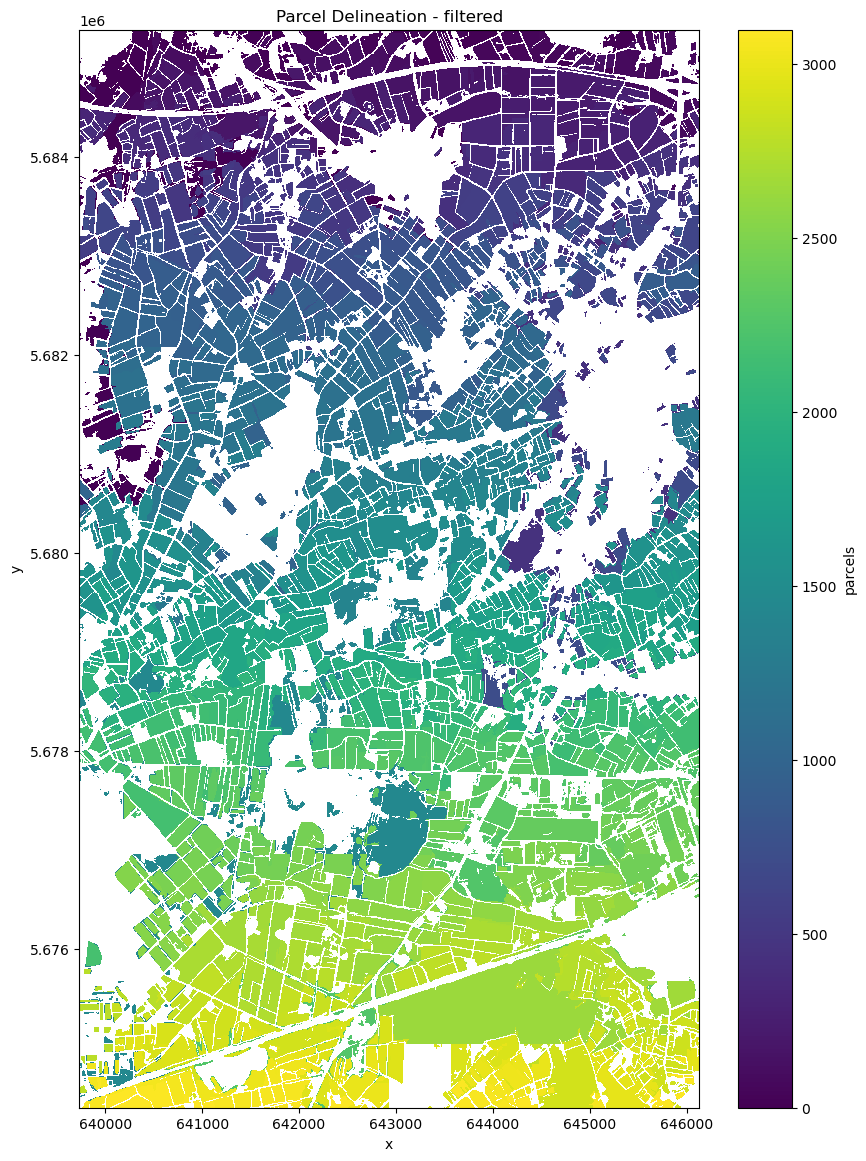
We present two different visualizations of the results. First one is a simple black and white plot of the results. The second is a segmentation used to highlight and delineate the parcels.
ds = xr.open_dataset("segmentation_result_parallel.nc")

ds.prediction.plot(figsize=(10, 14), cmap="gray")  # Use a colormap that suits your data
plt.title("Parcel Delineation")
plt.show()

## Close the dataset
ds.close()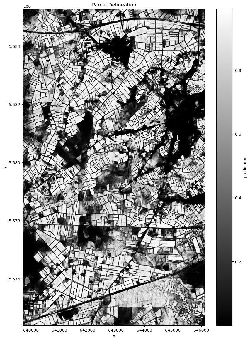
filtered = apply_filter(cube=ds.prediction, context={})

# Store the filtered result locally as netCDF
filtered.name = "parcels"
filtered.to_dataset().to_netcdf("segmentation_filtered")

## Plot the data
filtered.plot(figsize=(10, 14), cmap="viridis")  # Use a colormap that suits your data
plt.title("Parcel Delineation - filtered")
plt.show()

## Close the dataset
ds.close()
Dimensions of the final datacube ('time', 'y', 'x')