NDVI-based approach to study Landslide areas

Table of contents¶

Preface
Introduction
Setup
Data Access
Compute Reflectance and NDVI
Result Visualization

Preface¶

The original notebook used as a starting point for this work is a Copernicus Data Space Ecosystem example, available here.
The example has been adapted to use the data provided by the EOPF Zarr Samples project instead of the openEO API.

Introduction¶

Research indicates that NDVI can play a crucial role in identifying landslide zones. While an advanced workflow is possible, this notebook opts for a simple approach using the difference of NDVI and applying a threshold to the result to detect landslide occurred areas. Our analysis relies on the Sentinel-2 Level 2A data from the EOPF Sentinel Zarr Samples project.

Setup¶

Start importing the necessary libraries

import os
import xarray as xr
from datetime import datetime
import s3fs
from concurrent.futures import ThreadPoolExecutor, as_completed
from tqdm.auto import tqdm
from rasterio.plot import show
from typing import List
import rasterio
import matplotlib
import matplotlib.pyplot as plt
import matplotlib.patches as patches
from distributed import LocalCluster
import re
from pyproj import Transformer

Dask Cluster¶

Create Local Dask Cluster to access and process the data in parallel.

cluster = LocalCluster()
client = cluster.get_client()
client

Data Access¶

We now want to access a time series of Sentinel-2 data to compute the yearly NDVI index, remove cloudy pixels, and perform other processing steps.

List of available remote files¶

Here, we do the test for Ischia in Italy for the fall of 2022, where several landsides were registered.
The Sentinel-2 tiles covering the area are T33TVF and T33TUF and therefore we will query only the names containing the specific tile identifier.

In the cell below, we create a list of the matching Zarr files in the bucket.

bucket = "e05ab01a9d56408d82ac32d69a5aae2a:sample-data"
prefixes = ["tutorial_data/cpm_v253/", "tutorial_data/cpm_v256/"]
prefix_url = "https://objectstore.eodc.eu:2222"

fs = s3fs.S3FileSystem(anon=True, client_kwargs={"endpoint_url": prefix_url})

# Unregister handler for CEPH as before
handlers = fs.s3.meta.events._emitter._handlers
handlers_to_unregister = handlers.prefix_search("before-parameter-build.s3")
handler_to_unregister = handlers_to_unregister[0]
fs.s3.meta.events._emitter.unregister(
    "before-parameter-build.s3", handler_to_unregister
)

filtered_remote_files = []
for prefix in prefixes:
    # Include Sentinel-2 A and B for the specific tiles covering Ischia
    s3path_S2A_T33TUF = f"s3://{bucket}/{prefix}S2A*N0400*T33TUF*.zarr"
    s3path_S2A_T33TVF = f"s3://{bucket}/{prefix}S2A*N0400*T33TVF*.zarr"
    candidates = fs.glob(s3path_S2A_T33TUF) + fs.glob(s3path_S2A_T33TVF)
    for filepath in candidates:
        filtered_remote_files.append(filepath)

We want to use only the data for the specific temporal range before and after the landslide.
Hence, we specify the time ranges and filter the products based on their acquisition date.

post_start_date = datetime(2022, 11, 26).date()
post_end_date = datetime(2022, 12, 25).date()
pre_start_date = datetime(2022, 8, 25).date()
pre_end_date = datetime(2022, 11, 25).date()

def extract_date(filepath):
    match = re.search(r"S2A_MSIL2A_(\d{8})T\d{6}_N", filepath)
    return datetime.strptime(match.group(1), "%Y%m%d").date() if match else None


filtered_files_post = [
    f"{prefix_url}/{f.lstrip('/')}"
    for f in filtered_remote_files
    if (date := extract_date(f)) and (post_start_date <= date <= post_end_date)
]
filtered_files_pre = [
    f"{prefix_url}/{f.lstrip('/')}"
    for f in filtered_remote_files
    if (date := extract_date(f)) and (pre_start_date <= date <= pre_end_date)
]

Finally, we test if all the dataset can be opened correctly.

def check_dataset_availability(url):
    """
    Try opening the dataset using xr.open_datatree.
    Returns True if available, False otherwise.
    """
    try:
        xr.open_dataset(url, engine="zarr", chunks={})
        return True
    except FileNotFoundError:
        return False


# 2. Modified dataset processing with availability checks
def get_valid_datasets(datasets: List) -> List:
    """Process URLs and check availability in parallel"""

    # Check availability in parallel
    with ThreadPoolExecutor(max_workers=8) as executor:
        futures = {
            executor.submit(check_dataset_availability, ds): ds for ds in datasets
        }

        valid_datasets = []
        for future in tqdm(
            as_completed(futures), total=len(datasets), desc="Checking datasets"
        ):
            ds = futures[future]
            if future.result():
                valid_datasets.append(ds)

    print(f"Found {len(valid_datasets)}/{len(datasets)} valid datasets")
    return valid_datasets


pre_datasets = get_valid_datasets(filtered_files_pre)
post_datasets = get_valid_datasets(filtered_files_post)

Checking datasets:   0%|          | 0/34 [00:00<?, ?it/s]

Checking datasets: 100%|██████████| 34/34 [00:00<00:00, 131.51it/s]

Found 34/34 valid datasets

Checking datasets: 100%|██████████| 4/4 [00:00<00:00, 29.01it/s]

Found 4/4 valid datasets

Data Cube Building¶

We can now create a Data Cube (which consist in an Xarray Dataset object) containing the full timeseries for the two selected temporal ranges, before and after the landslide.

We firstly convert the Area of Interest (AOI), given in EPSG:4326 coordinates, to the target Coordinate Reference System (CRS) of the selected Sentinel-2 data, which correspond to EPSG:32633.

ds = xr.open_datatree(pre_datasets[0], engine="zarr", chunks={}, decode_timedelta=False)
target_crs = ds.attrs["stac_discovery"]["properties"]["proj:epsg"]
print(f"Target CRS of the selected Sentinel-2 tiles: {target_crs}")

# Define AOI and convert to raster CRS
spatial_extent = {
    "west": 13.882567409197492,
    "south": 40.7150627793427,
    "east": 13.928593792166282,
    "north": 40.747050251559216,
}
# Convert AOI to UTM 33N (same as Sentinel-2 data)
transformer = Transformer.from_crs("EPSG:4326", "EPSG:32633", always_xy=True)
west_utm, south_utm = transformer.transform(
    spatial_extent["west"], spatial_extent["south"]
)
east_utm, north_utm = transformer.transform(
    spatial_extent["east"], spatial_extent["north"]
)

# Spatial slice parameters
x_slice = slice(west_utm, east_utm)
y_slice = slice(north_utm, south_utm)

Target CRS of the selected Sentinel-2 tiles: 32633

We now define an utility function which will extract the product date and assign it as a coordinate at loading time, which is necessary to stack the products along time.
Moreover, again at loading time, the data will also be cropped to the defined AOI over Ischia.

def extract_time_and_crop(ds):
    date_format = "%Y%m%dT%H%M%S"
    filename = ds.encoding["source"]
    date_str = os.path.basename(filename).split("_")[2]
    time = datetime.strptime(date_str, date_format)
    ds = ds.assign_coords(time=time)
    return ds.sel(x=x_slice, y=y_slice)

%%time
r10m_pre = xr.open_mfdataset(
    pre_datasets,
    engine="zarr",
    chunks={},
    group="/measurements/reflectance/r10m",
    concat_dim="time",
    combine="nested",
    preprocess=extract_time_and_crop,
    decode_cf=False,
    mask_and_scale=False,
)
r10m_pre.rio.write_crs(target_crs, inplace=True)
r10m_pre

%%time
r10m_post = xr.open_mfdataset(
    post_datasets,
    engine="zarr",
    chunks={},
    group="/measurements/reflectance/r10m",
    concat_dim="time",
    combine="nested",
    preprocess=extract_time_and_crop,
    decode_cf=False,
    mask_and_scale=False,
)
r10m_post.rio.write_crs(target_crs, inplace=True)
r10m_post

The area of Ischia lies exactly in the overlapping part of two Sentinel-2 tiles. To harmonize the Data Cube along time, so that it contains only a slice per unique date, we will now use the groupy operator of Xarray. Notice the change in the number of labels along the time dimension after this operation.

r10m_pre = (
    r10m_pre.groupby(r10m_pre.time.dt.floor("D"))
    .mean(skipna=True)
    .rename({"floor": "time"})
)
r10m_post = (
    r10m_post.groupby(r10m_post.time.dt.floor("D"))
    .mean(skipna=True)
    .rename({"floor": "time"})
)
r10m_pre

Compute Reflectance and NDVI¶

Before computing the average Normalized Difference Vegetation Index (NDVI) over time, we need to compute reflectance values.

To compute Bottom of Atmosphere Reflectance (BOA) values from the digital numbers (DNs) from original Sentinel SAFE data we would need to rescale the data following this formula:

$L2A\_BOA = (L2A\_DN + BOA\_ADD\_OFFSET) / BOA\_QUANTIFICATION\_VALUE$

where BOA_ADD_OFFSET = -1000 and BOA_QUANTIFICATION_VALUE = 10000
ESA Reference: https://sentinels.copernicus.eu/web/sentinel/-/copernicus-sentinel-2-major-products-upgrade-upcoming

However, the scale and offset parameters in the Zarr metadata have been adapted so that Xarray can rescale the data automatically (setting mask_and_scale=True) and therefore the formula to get reflectance values is:
$L2A\_BOA = (L2A\_ZARR\_VALUE * scale\_factor) + add\_offset$

where add_offset = -0.1 and scale_factor = 0.0001
ESA EOPF reference: https://cpm.pages.eopf.copernicus.eu/eopf-cpm/main/PSFDjan2024.html#scaling

def calculate_ndvi(ds: xr.Dataset) -> xr.DataArray:
    """Calculate NDVI from dataset with B04 and B08"""
    red = (ds["b04"] * ds["b04"].attrs["_eopf_attrs"]["scale_factor"]) + ds[
        "b04"
    ].attrs["_eopf_attrs"]["add_offset"]

    nir = (ds["b08"] * ds["b08"].attrs["_eopf_attrs"]["scale_factor"]) + ds[
        "b08"
    ].attrs["_eopf_attrs"]["add_offset"]

    return (nir - red) / (nir + red)


pre_ndvi = calculate_ndvi(r10m_pre).mean(dim="time")
post_ndvi = calculate_ndvi(r10m_post).mean(dim="time")

We finally compute the NDVI difference and save it as a geoTIFF.

ndvi_diff = post_ndvi - pre_ndvi
ndvi_diff.rio.to_raster("NDVI_diff_Ischia_landslide.tiff")

/home/mclaus@eurac.edu/micromamba/envs/eopf-zarr/lib/python3.11/site-packages/dask/core.py:127: RuntimeWarning: divide by zero encountered in divide
  return func(*(_execute_task(a, cache) for a in args))

Result Visualization¶

img = rasterio.open("NDVI_diff_Ischia_landslide.tiff")
value = img.read(1)
cmap = matplotlib.colors.ListedColormap(["black", "red"])
fig, ax = plt.subplots(figsize=(8, 6), dpi=80)

show(((value < -0.3) & (value > -1)), cmap=cmap, transform=img.transform, ax=ax)
ax.set_title("Detected Landslide Area")
ax.set_xlabel("X Coordinates")
ax.set_ylabel("Y Coordinates")


area = [
    patches.Patch(color=color, label=label)
    for color, label in zip(["black", "red"], ["Absence", "Presence"])
]
fig.legend(handles=area, bbox_to_anchor=(0.83, 1.03), loc=1)
plt.show()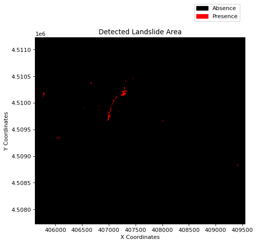

A general observation drawn from the aforementioned result is that the red regions indicate potential landslide activity or vegetation loss.

The red region corresponds to an area where notably large landslides were recorded. However, some false positives can also be noticed in the northwest—an urban area, though not many landslides were reported in those regions. Hence, it is conceivable that there is a change in NDVI, but it might be due to many factors, such as cloud cover, harvesting, vegetation loss, etc. This shows that the difference in the NDVI approach is suitable for rapid mapping but can also contain a lot of misclassified pixels and needs further validation.

client.close()

Jupyter Notebooks

Deforestation Monitoring using Sentinel 2 and xarray

Jupyter Notebooks

Introduction to xarray-eopf backend.