Deforestation Monitoring using Sentinel 2 and xarray
Streamlining Cloud-Based Processing with EOPF and Xarray

Table of contents
Run this notebook interactively with all dependencies pre-installed
Preface
The original notebook used as a starting point for this work is a Copernicus Data Space Ecosystem example, available here.
The example has been adapted to use the data provided by the EOPF Zarr Samples project instead of the openEO API.
Introduction
Sentinel-2 data is one of the most widely used satellite datasets, but working with it still presents several challenges. To obtain analysis-ready data, users often need to generate cloud-free mosaics.
Accessing large volumes of data through tiles can be time-consuming, and preparing the data in formats compatible with common Python tools is not always straightforward.
In this notebook, we demonstrate how accessing and preparing Sentinel-2 data for analysis in Python can be streamlined when the data is available in the EOPF Zarr format and used within the EOPF Sample Service JupyterHub environment. We walk through a basic deforestation monitoring use case, leveraging the powerful xarray library to efficiently handle and explore the multidimensional satellite data.
Setup
Start importing the necessary libraries
import os
import s3fs
from datetime import datetime
from pathlib import Path

import geopandas as gpd
import matplotlib.colors as mcolors
import matplotlib.patches as mpatches
import matplotlib.pyplot as plt
import numpy as np
import requests
import xarray as xr
from shapely import geometry

# Set up a local cluster for distributed computing.
from distributed import LocalCluster
Set up a local cluster for distributed computing.
cluster = LocalCluster()
client = cluster.get_client()
client
/home/mclaus@eurac.edu/micromamba/envs/eopf-zarr3/lib/python3.11/site-packages/distributed/node.py:187: UserWarning: Port 8787 is already in use.
Perhaps you already have a cluster running?
Hosting the HTTP server on port 37147 instead
warnings.warn(
Data Access
We now want to access a time series in order to compute the yearly NDVI index, remove cloudy pixels, and perform other processing steps.
List of available remote files
Let’s make a list of available files for this example. In the cell below, we list the available Zarr files in the bucket and print the first five filenames.
bucket = "e05ab01a9d56408d82ac32d69a5aae2a:sample-data"
prefix = "tutorial_data/cpm_v253/"
prefix_url = "https://objects.eodc.eu"
# Create the S3FileSystem with a custom endpoint
fs = s3fs.S3FileSystem(anon=True, client_kwargs={"endpoint_url": prefix_url})

# unregister handler to make boto3 work with CEPH
handlers = fs.s3.meta.events._emitter._handlers
handlers_to_unregister = handlers.prefix_search("before-parameter-build.s3")
handler_to_unregister = handlers_to_unregister[0]
fs.s3.meta.events._emitter.unregister(
    "before-parameter-build.s3", handler_to_unregister
)

s3path = "s3://" + f"{bucket}/{prefix}" + "S2A_MSIL2A_*_*_*_T32UPC_*.zarr"

remote_files = fs.glob(s3path)

remote_product_path = prefix + remote_files[0]
paths = [f"{prefix_url}/{f}" for f in remote_files]
paths[:5]
['https://objects.eodc.eu/e05ab01a9d56408d82ac32d69a5aae2a:sample-data/tutorial_data/cpm_v253/S2A_MSIL2A_20180601T102021_N0500_R065_T32UPC_20230902T045008.zarr',
'https://objects.eodc.eu/e05ab01a9d56408d82ac32d69a5aae2a:sample-data/tutorial_data/cpm_v253/S2A_MSIL2A_20180604T103021_N0500_R108_T32UPC_20230819T205634.zarr',
'https://objects.eodc.eu/e05ab01a9d56408d82ac32d69a5aae2a:sample-data/tutorial_data/cpm_v253/S2A_MSIL2A_20180611T102021_N0500_R065_T32UPC_20230714T225353.zarr',
'https://objects.eodc.eu/e05ab01a9d56408d82ac32d69a5aae2a:sample-data/tutorial_data/cpm_v253/S2A_MSIL2A_20180614T103021_N0500_R108_T32UPC_20230813T122609.zarr',
'https://objects.eodc.eu/e05ab01a9d56408d82ac32d69a5aae2a:sample-data/tutorial_data/cpm_v253/S2A_MSIL2A_20180621T102021_N0500_R065_T32UPC_20230827T073006.zarr']Procedure to compute cloudless NDVI
Select the classification map variable (scl) to mask invalid pixels (e.g., no data, saturated, cloudy).
Since the scl variable is available at a different spatial resolution (20m), it is interpolated to 10m resolution.
Then, compute a cloud-free NDVI using the B04 and B08 bands.
Full Timeseries Data Cube
To create a Data Cube containing the full timeseries, we need to extract the time information.
We use the file name to get the date and time information.
def extract_time(ds):
    date_format = "%Y%m%dT%H%M%S"
    filename = ds.encoding["source"]
    date_str = os.path.basename(filename).split("_")[2]
    time = datetime.strptime(date_str, date_format)
    return ds.assign_coords(time=time)
%%time
r10m = xr.open_mfdataset(
paths,
engine="zarr",
chunks={},
group="/measurements/reflectance/r10m",
concat_dim="time",
combine="nested",
preprocess=extract_time,
decode_cf=False,
mask_and_scale=False,
)
r10m/home/mclaus@eurac.edu/micromamba/envs/eopf-zarr3/lib/python3.11/site-packages/xarray_sentinel/esa_safe.py:7: UserWarning: pkg_resources is deprecated as an API. See https://setuptools.pypa.io/en/latest/pkg_resources.html. The pkg_resources package is slated for removal as early as 2025-11-30. Refrain from using this package or pin to Setuptools<81.
import pkg_resources
CPU times: user 3.65 s, sys: 468 ms, total: 4.12 s
Wall time: 25.7 s
%%time
r20m_mask_l2a_classification = xr.open_mfdataset(
    paths,
    engine="zarr",
    chunks={},
    group="conditions/mask/l2a_classification/r20m",
    concat_dim="time",
    combine="nested",
    preprocess=extract_time,
    decode_cf=False,
    mask_and_scale=False,
)
r20m_mask_l2a_classification
CPU times: user 2.63 s, sys: 376 ms, total: 3 s
Wall time: 19.6 s
Set desired resolution of our data
To speed up the processing, we resample the data to a coarsen resolution, i.e. 100m.
# Define the resampling factor (10m to 100m = 10x)
factor = 10
r100m = r10m.coarsen(x=factor, y=factor, boundary="trim").mean()
r100mStart computing
Masking
Firstly resample the SCL layer the same resolution as B02, B03, B04, B08 and apply the mask per pixel
%%time
scl_100m = (
    r20m_mask_l2a_classification.scl.chunk(chunks={"x": -1, "y": -1}).interp(
        x=r100m["x"], y=r100m["y"], method="nearest"
    )
    # Copy chunking from r10m['b02'] to cls_r10m
    .chunk(r100m["b02"].chunks)
)
scl_100m
CPU times: user 612 ms, sys: 5.94 ms, total: 618 ms
Wall time: 636 ms
<timed exec>:6: DeprecationWarning: Supplying chunks as dimension-order tuples is deprecated. It will raise an error in the future. Instead use a dict with dimension names as keys.
Create a boolean mask based on the labels we consider (clouds high probability, cloud shadows, no data, ...)
def validate_scl(scl):
    invalid = [0, 1, 3, 7, 8, 9, 10]  # NO_DATA, SATURATED, CLOUD, etc.
    return ~scl.isin(invalid)


valid_mask = validate_scl(scl_100m)  # Boolean mask (10980x10980)
valid_maskApply the mask to the data cube:
valid_r100m = r100m.where(valid_mask)
valid_r100mScaling
Apply scale factor and add offset (i.e. Digital Numbers to Reflenctances conversion). Note: the scale and offset are the same for all the B1 - B12 bands.
scale = valid_r100m["b04"].attrs["_eopf_attrs"]["scale_factor"]
offset = valid_r100m["b08"].attrs["_eopf_attrs"]["add_offset"]
reflectances_r100m = (valid_r100m * scale) + offset
Compute the NDVI and stack the result with the cloudless bands
b08 = reflectances_r100m["b08"]
b04 = reflectances_r100m["b04"]
ndvi = (b08 - b04) / (b08 + b04)  # Per-pixel NDVI
reflectances_r100m["ndvi"] = ndvi
reflectances_r100mIndexing and selecting data
Select one date
cloudless_bands_ndvi = reflectances_r100m.sel(
    time=datetime(2018, 6, 4), method="nearest"
)
Subset spatially
It is always good practice to select data over the area of interest, as this can significantly reduce memory usage when computing NDVI or applying any processing.
epsg = 32632  # Sentinel-2 data CRS known a priori

bbox = [10.633501, 51.611195, 10.787234, 51.698098]
bbox_polygon = geometry.box(*bbox)
polygon = gpd.GeoDataFrame(index=[0], crs="epsg:4326", geometry=[bbox_polygon])
polygon.explore()Reproject the bbox to the target Sentinel-2 UTM projection:
bbox_reproj = polygon.to_crs("epsg:" + str(epsg)).geometry.values[0].bounds
bbox_reproj
(612890.0057926236, 5719059.568597787, 623750.1130221735, 5728972.640384748)Take a subset of ~100x100 pixels:
x_slice = slice(bbox_reproj[0], bbox_reproj[2])  # ~100 pixels
y_slice = slice(bbox_reproj[3], bbox_reproj[1])  # ~100 pixels

region = cloudless_bands_ndvi.sel(x=x_slice, y=y_slice).chunk(
    {"y": "auto", "x": "auto"}
)
regionPlot NDVI & RGB
Load in memory RGB and NDVI for a selected time and geographical area
%%time
rgb = region[["b04", "b03", "b02"]].to_dataarray(dim="bands")
rgb = (rgb - 0.02) / (0.35 - 0.02)  # Stretch 0.02-0.35 to 0-1
rgb = rgb.clip(0, 1).compute()
ndvi = region["ndvi"].compute()
/home/mclaus@eurac.edu/micromamba/envs/eopf-zarr3/lib/python3.11/site-packages/distributed/client.py:3363: UserWarning: Sending large graph of size 44.93 MiB.
This may cause some slowdown.
Consider loading the data with Dask directly
or using futures or delayed objects to embed the data into the graph without repetition.
See also https://docs.dask.org/en/stable/best-practices.html#load-data-with-dask for more information.
warnings.warn(
/home/mclaus@eurac.edu/micromamba/envs/eopf-zarr3/lib/python3.11/site-packages/distributed/client.py:3363: UserWarning: Sending large graph of size 43.85 MiB.
This may cause some slowdown.
Consider loading the data with Dask directly
or using futures or delayed objects to embed the data into the graph without repetition.
See also https://docs.dask.org/en/stable/best-practices.html#load-data-with-dask for more information.
warnings.warn(
CPU times: user 5.39 s, sys: 231 ms, total: 5.62 s
Wall time: 7.86 s
fig, (ax1, ax2) = plt.subplots(1, 2, figsize=(12, 5))
fig.suptitle("Date - 20180604T103021\n")

# First subplot
rgb.plot.imshow(
    ax=ax1,
    rgb="bands",
    extent=(x_slice.start, x_slice.stop, y_slice.start, y_slice.stop),
)

ax1.set_title("RGB (Enhanced)")

# Second plot
ndvi_plot = ndvi.plot(ax=ax2, cmap="Greens", vmin=-1, vmax=1, add_colorbar=False)
ax2.set_title("NDVI")

# Add color bar on the right
fig.subplots_adjust(right=0.8)
cbar_ax = fig.add_axes([0.85, 0.15, 0.05, 0.7])
fig.colorbar(ndvi_plot, cax=cbar_ax)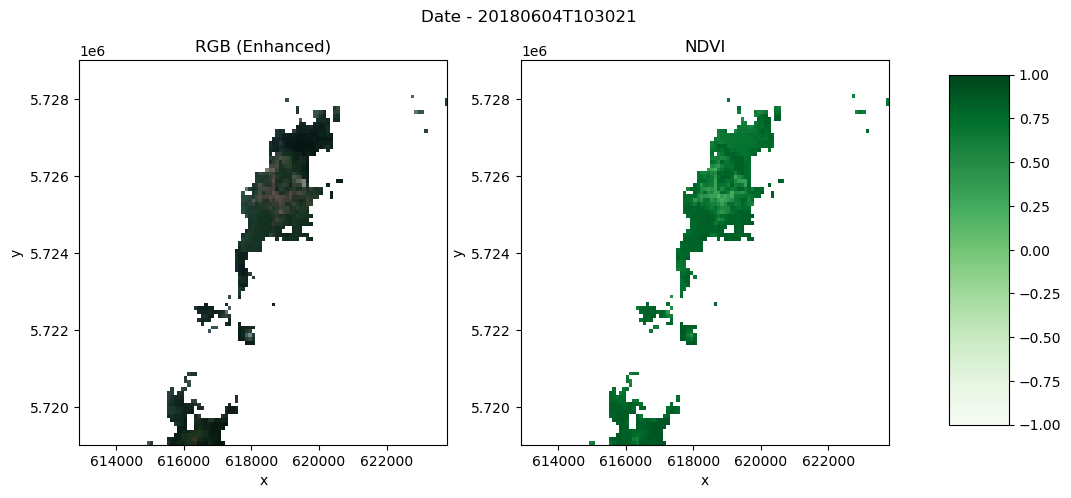
Yearly mean
# Group by year and compute mean
yearly_ds = (
    reflectances_r100m.sel(x=x_slice, y=y_slice)
    .groupby("time.year")
    .mean(dim="time", skipna=True)
)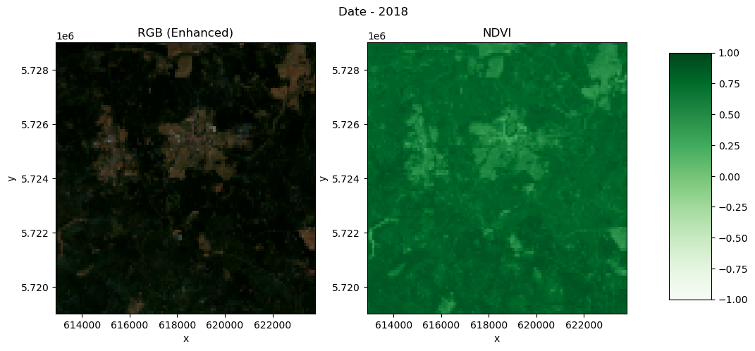
yearly_dsVisualize NDVI for 2018
def plot_rgb_ndvi(dset, year, x_slice, y_slice):
    fig, (ax1, ax2) = plt.subplots(1, 2, figsize=(12, 5))
    fig.suptitle("Date - " + str(year) + "\n")

    # First subplot
    rgb = dset[["b04", "b03", "b02"]].to_dataarray(dim="bands")
    rgb = (rgb - 0.02) / (0.35 - 0.02)  # Stretch 0.02-0.35 to 0-1
    rgb = rgb.clip(0, 1)  # Clip to valid range
    rgb.plot.imshow(
        ax=ax1,
        rgb="bands",
        extent=(x_slice.start, x_slice.stop, y_slice.start, y_slice.stop),
    )
    ax1.set_title("RGB (Enhanced)")

    # Second plot
    ndvi_plot = dset["ndvi"].plot(
        ax=ax2, cmap="Greens", vmin=-1, vmax=1, add_colorbar=False
    )
    ax2.set_title("NDVI")

    # Add color bar on the right
    fig.subplots_adjust(right=0.8)
    cbar_ax = fig.add_axes([0.85, 0.15, 0.05, 0.7])
    fig.colorbar(ndvi_plot, cax=cbar_ax)
year = 2018
region = yearly_ds.sel(year=year)
plot_rgb_ndvi(region, year, x_slice, y_slice)/home/mclaus@eurac.edu/micromamba/envs/eopf-zarr3/lib/python3.11/site-packages/distributed/client.py:3363: UserWarning: Sending large graph of size 45.13 MiB.
This may cause some slowdown.
Consider loading the data with Dask directly
or using futures or delayed objects to embed the data into the graph without repetition.
See also https://docs.dask.org/en/stable/best-practices.html#load-data-with-dask for more information.
warnings.warn(
/home/mclaus@eurac.edu/micromamba/envs/eopf-zarr3/lib/python3.11/site-packages/distributed/client.py:3363: UserWarning: Sending large graph of size 43.92 MiB.
This may cause some slowdown.
Consider loading the data with Dask directly
or using futures or delayed objects to embed the data into the graph without repetition.
See also https://docs.dask.org/en/stable/best-practices.html#load-data-with-dask for more information.
warnings.warn(
Visualise NDVI from 2018 to 2023
ndvi_yearly = yearly_ds["ndvi"].sel(x=x_slice, y=y_slice).sel(year=slice(2018, 2023))

ndvi_yearly.plot(
    cmap="PRGn", x="x", y="y", col="year", col_wrap=2, vmin=-1, vmax=1, figsize=(10, 15)
)
/home/mclaus@eurac.edu/micromamba/envs/eopf-zarr3/lib/python3.11/site-packages/distributed/client.py:3363: UserWarning: Sending large graph of size 43.92 MiB.
This may cause some slowdown.
Consider loading the data with Dask directly
or using futures or delayed objects to embed the data into the graph without repetition.
See also https://docs.dask.org/en/stable/best-practices.html#load-data-with-dask for more information.
warnings.warn(
<xarray.plot.facetgrid.FacetGrid at 0x7fbaa6586490>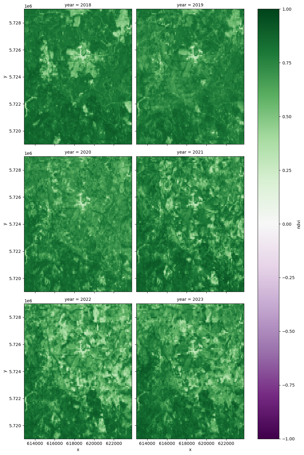
Saving data into local Zarr
Prepare the dataset to be saved with a particular attention to chunks
region = region.chunk({"y": 50, "x": 55})
print(region.chunks)
Frozen({'y': (50, 50), 'x': (55, 54)})
Write the data to Zarr, setting the data type to float32 to reduce the storage need:
%%time
encoding = {}
for var in region.data_vars:
    encoding[var] = {"dtype": "float32"}
region.to_zarr("data_region.zarr", zarr_format=2, encoding=encoding, mode="w")
<timed exec>:4: SerializationWarning: saving variable None with floating point data as an integer dtype without any _FillValue to use for NaNs
<timed exec>:4: SerializationWarning: saving variable None with floating point data as an integer dtype without any _FillValue to use for NaNs
/home/mclaus@eurac.edu/micromamba/envs/eopf-zarr3/lib/python3.11/site-packages/distributed/client.py:3363: UserWarning: Sending large graph of size 46.35 MiB.
This may cause some slowdown.
Consider loading the data with Dask directly
or using futures or delayed objects to embed the data into the graph without repetition.
See also https://docs.dask.org/en/stable/best-practices.html#load-data-with-dask for more information.
warnings.warn(
CPU times: user 6.05 s, sys: 430 ms, total: 6.48 s
Wall time: 15.9 s
<xarray.backends.zarr.ZarrStore at 0x7fbaa29fd300>The stored Zarr data could be further reused in a subsequent analysis offline. This is especially useful if you need to interact, visualize and experiment with the data intensively and would avoid to download the data multiple times from the cloud storage.
Analysis
For analysis the first step is to classify pixels as forest. In our case we will just do a simple thresholding classification where we classify everything above a certain threshold as forest. This isn’t the best approach for classifying forest, since agricultural areas can also easily reach very high NDVI values. A better approach would be to classify based on the temporal signature of the pixel.
However, for this basic analysis, we stick to the simple thresholding approach.
In this case we classify everything above an NDVI of 0.7 as forest. This calculated forest mask is then saved to a new Data Variable in the xarray dataset:
yearly_ds["FOREST"] = yearly_ds.ndvi > 0.7With this forest mask we can already do a quick preliminary analysis to plot the total forest area over the years.
To do this we sum up the pixels along the x and y coordinate but not along the time coordinate. This will leave us with one value per year representing the number of pixels classified as forest. We can then calculate the forest area by multiplying the number of forest pixels by the resolution.
def to_km2(dataarray, resolution):
    # Calculate forest area
    return dataarray * np.prod(list(resolution)) / 1e6
resolution = (100, 100)
forest_pixels = yearly_ds.sel(x=x_slice, y=y_slice).FOREST.sum(["x", "y"])
forest_area_km2 = to_km2(forest_pixels, resolution)
forest_area_km2forest_area_km2.load()/home/mclaus@eurac.edu/micromamba/envs/eopf-zarr3/lib/python3.11/site-packages/distributed/client.py:3363: UserWarning: Sending large graph of size 43.92 MiB.
This may cause some slowdown.
Consider loading the data with Dask directly
or using futures or delayed objects to embed the data into the graph without repetition.
See also https://docs.dask.org/en/stable/best-practices.html#load-data-with-dask for more information.
warnings.warn(
forest_area_km2.plot()

plt.title("Forest Cover")
plt.ylabel("Forest Cover [km²]")
plt.ylim(0);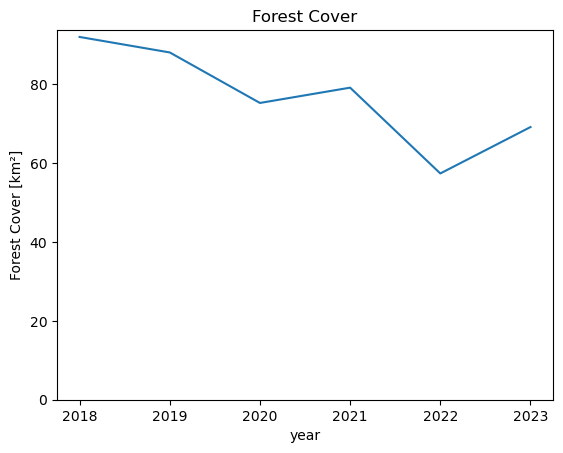
We can see that the total forest area in this AOI decreased from around 80 km² in 2018 to only around 50 km² in 2023.
The next step is to make change maps from year to year. To do this we basically take the difference of the forest mask of a year with its previous year.
This will result in 0 value where there has been no change, -1 where forest was lost and +1 where forest was gained.
# Make change maps of forest loss and forest gain compared to previous year

# 0 - 0 = No Change: 0
# 1 - 1 = No Change: 0
# 1 - 0 = Forest Gain: 1
# 0 - 1 = Forest Loss: -1

# Define custom colors and labels
colors = ["darkred", "white", "darkblue"]
labels = ["Forest Loss", "No Change", "Forest Gain"]

# Create a colormap and normalize it
cmap = mcolors.ListedColormap(colors)
norm = plt.Normalize(-1, 1)  # Adjust the range based on your data
Use 2022 as plot_year
plot_year = 2022
yearly_ds["CHANGE"] = yearly_ds.FOREST.astype(int).diff("year", label="upper")yearly_ds["CHANGE"].compute()/home/mclaus@eurac.edu/micromamba/envs/eopf-zarr3/lib/python3.11/site-packages/distributed/client.py:3363: UserWarning: Sending large graph of size 43.93 MiB.
This may cause some slowdown.
Consider loading the data with Dask directly
or using futures or delayed objects to embed the data into the graph without repetition.
See also https://docs.dask.org/en/stable/best-practices.html#load-data-with-dask for more information.
warnings.warn(
Visualize the differences
yearly_ds.CHANGE.sel(year=plot_year).plot(cmap=cmap, norm=norm, add_colorbar=False)
# Create a legend with string labels
legend_patches = [
    mpatches.Patch(color=color, label=label) for color, label in zip(colors, labels)
]
plt.legend(handles=legend_patches, loc="lower left")
plt.title(f"Forest Change Map {plot_year}");
/home/mclaus@eurac.edu/micromamba/envs/eopf-zarr3/lib/python3.11/site-packages/distributed/client.py:3363: UserWarning: Sending large graph of size 43.93 MiB.
This may cause some slowdown.
Consider loading the data with Dask directly
or using futures or delayed objects to embed the data into the graph without repetition.
See also https://docs.dask.org/en/stable/best-practices.html#load-data-with-dask for more information.
warnings.warn(
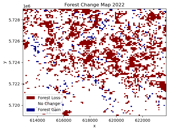
Here, we can see the spatial distribution of areas affected by forest loss. In the displayed change from 2021 to 2022, most of the forest loss happened in the northern part of the study area, while the southern part lost comparatively less forest.
To get a feel for the loss per year, we can cumulatively sum up the lost areas over the years. This should basically follow the same trends as the earlier plot of total forest area.
# Forest Loss per Year
forest_loss = (yearly_ds.CHANGE == -1).sum(["x", "y"])
forest_loss_km2 = to_km2(forest_loss, resolution)
forest_loss_km2.cumsum().plot()
plt.title("Cumulative Forest Loss")
plt.ylabel("Forest Loss [km²]");
/home/mclaus@eurac.edu/micromamba/envs/eopf-zarr3/lib/python3.11/site-packages/distributed/client.py:3363: UserWarning: Sending large graph of size 43.93 MiB.
This may cause some slowdown.
Consider loading the data with Dask directly
or using futures or delayed objects to embed the data into the graph without repetition.
See also https://docs.dask.org/en/stable/best-practices.html#load-data-with-dask for more information.
warnings.warn(
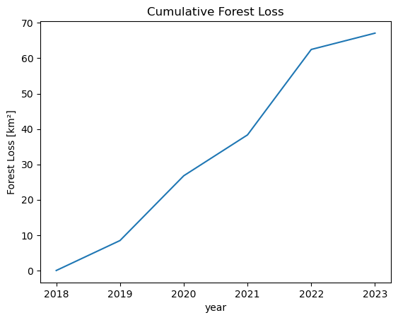
We can see that there have been two years with particularly large amounts of lost forest area. From 2019-2020 and with by far the most lost area between 2021 and 2022.
Validation
Finally, we want to see how accurate our data is compared to the widely used Hansen Global Forest Change data. In a real scientific scenario, we would use Ground Truth data to assess the accuracy of our classification. In this case we use the Global Forest Change data in place of Ground Truth data, just to show how an accuracy assessment can be done. The assessment we are doing only shows how accurately we replicate the Global Forest Change data, however we will not know if our product is more or less accurate. For a more accurate assessment, actual Ground Truth data is required.
First we download the Global Forest Change Data here and open it using Xarray.
data_path = Path("./data/")
data_path.mkdir(parents=True, exist_ok=True)
hansen_filename = "Hansen_GFC-2022-v1.10_lossyear_60N_010E.tif"
comp_data = data_path / hansen_filename

with comp_data.open("wb") as fs:
    hansen_data = requests.get(
        f"https://storage.googleapis.com/earthenginepartners-hansen/GFC-2022-v1.10/{hansen_filename}"
    )
    fs.write(hansen_data.content)
import matplotlib.pyplot as plt
import rioxarray
target_epsg = epsg
# Open the file (replace 'comp_data' with your raster file path)
ground_truth = (
rioxarray.open_rasterio(comp_data) # Replace with your file path
.rio.clip_box(
minx=bbox[0],
miny=bbox[1],
maxx=bbox[2],
maxy=bbox[3],
)
.rio.reproject(target_epsg)
.sel(band=1)
.where(lambda gt: gt < 100, 0) # Fill no-data (values > 100) with 0
)
# Plot
ground_truth.plot(levels=range(25), cbar_kwargs={"label": "Year of Forest Loss"})
plt.title("Global Forest Watch Data")
plt.show()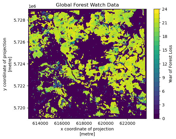
The data shows in which year forest was first lost. To compare with our own data, we need to add the data to our dataset. To do this the data needs to have the same coordinates. This can be achieved with .interp_like(). This function interpolates the data to match up the coordinates of another dataset.
In this case we chose the interpolation method nearest since it is categorical data.
yearly_ds["GROUND_TRUTH"] = ground_truth.interp_like(
    yearly_ds, method="nearest"
).astype(int)
yearly_ds
/home/mclaus@eurac.edu/micromamba/envs/eopf-zarr3/lib/python3.11/site-packages/xarray/core/duck_array_ops.py:243: RuntimeWarning: invalid value encountered in cast
return data.astype(dtype, **kwargs)
The ground truth data saves the year when deforestation was first detected for a pixel in a single raster. To do this, it encodes the year of forest loss as an integer, giving the year. So, an integer 21 means the pixel was first detected as deforested in 2021, whereas a value of 0 means that deforestation was never detected.
Currently our classification saves the deforestation detection in multiple rasters, one for each year. To get our data into a format that is similar to our comparison data we need to convert our rasters for each time step into a single one.
To do this we first assign all pixels which were detected as deforestation (CHANGE == -1) to the year in which the deforestation was detected (lost_year). Then we compute over our time-series the first occurence of deforestation (equivalent to the first non-zero value) per pixel. This is then saved in a new data variable.
# convert lost forest (-1) into the year it was lost
lost_year = (yearly_ds.CHANGE == -1) * yearly_ds.year % 100
first_nonzero = (lost_year != 0).argmax(axis=0).compute()
yearly_ds["LOST_YEAR"] = lost_year[first_nonzero]
yearly_ds.LOST_YEAR.plot(levels=range(25), cbar_kwargs={"label": "Year of Forest Loss"})
plt.title("Classification Forest Loss Year");
/home/mclaus@eurac.edu/micromamba/envs/eopf-zarr3/lib/python3.11/site-packages/distributed/client.py:3363: UserWarning: Sending large graph of size 43.94 MiB.
This may cause some slowdown.
Consider loading the data with Dask directly
or using futures or delayed objects to embed the data into the graph without repetition.
See also https://docs.dask.org/en/stable/best-practices.html#load-data-with-dask for more information.
warnings.warn(
/home/mclaus@eurac.edu/micromamba/envs/eopf-zarr3/lib/python3.11/site-packages/distributed/client.py:3363: UserWarning: Sending large graph of size 44.00 MiB.
This may cause some slowdown.
Consider loading the data with Dask directly
or using futures or delayed objects to embed the data into the graph without repetition.
See also https://docs.dask.org/en/stable/best-practices.html#load-data-with-dask for more information.
warnings.warn(
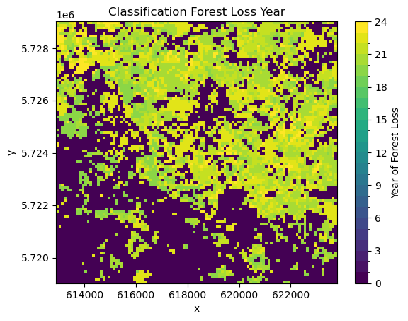
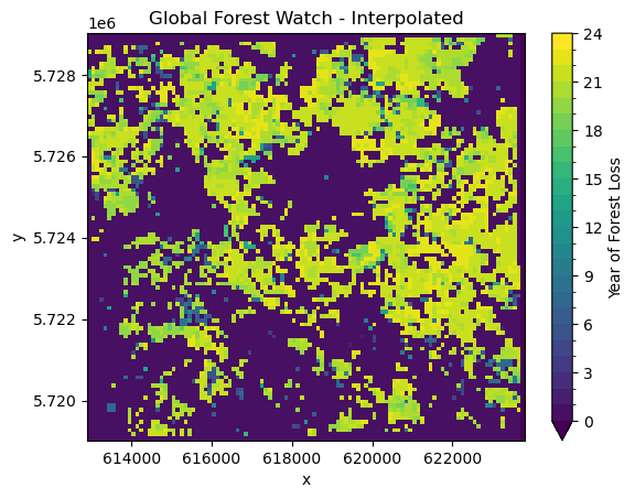
Comparing this visually to the Global Forest Watch data, allows us to do some initial quality assessment. We can see definite differences between the two datasets. The Global Forest Watch data has much more clearly defined borders. In general, our classification seems to overestimate deforestation. However, the general pattern of forest loss is the same in both. Most of the deforestation is in the north of the study area, with less forest loss in the south.
There are a few reasons for those differences. The main difference has to be in our much more simple approach to forest classification and change detection. It is expected that our approach will lead to large amounts of commission errors since changes are only confirmed using a single observation. It however can also lead to a lot of omission errors since the NDVI thresholding might classify highly productive non-forest areas as forest due to their high NDVI values.
However, there are also some systematic differences. Our algorithm looks at differences between the middle of the years, which means that some changes can happen at the end of the growing year which will be detected first in the next year whereas the Global Forest Watch dataset will detect it in the correct (earlier) year.
yearly_ds.GROUND_TRUTH.plot(
    levels=range(25), cbar_kwargs={"label": "Year of Forest Loss"}, cmap="viridis"
)
plt.title("Global Forest Watch - Interpolated");
/home/mclaus@eurac.edu/micromamba/envs/eopf-zarr3/lib/python3.11/site-packages/xarray/plot/utils.py:258: RuntimeWarning: overflow encountered in scalar absolute
vlim = max(abs(vmin - center), abs(vmax - center))
Finally, we can also calculate an accuracy score. This is a score from 0-1, where values close to 0.5 basically mean that the classification is random, and values close to 1 mean that most of the values of our comparison data and classification data match.
First, we look at the overall accuracy of forest loss over the entire period from 2018 to 2023.
from sklearn.metrics import accuracy_score

score = accuracy_score(
    (yearly_ds.LOST_YEAR > 18).values.ravel(),
    (yearly_ds.GROUND_TRUTH > 18).values.ravel(),
)
print(f"The overall accuracy of forest loss detection is {score:.2f}.")
/home/mclaus@eurac.edu/micromamba/envs/eopf-zarr3/lib/python3.11/site-packages/distributed/client.py:3363: UserWarning: Sending large graph of size 44.00 MiB.
This may cause some slowdown.
Consider loading the data with Dask directly
or using futures or delayed objects to embed the data into the graph without repetition.
See also https://docs.dask.org/en/stable/best-practices.html#load-data-with-dask for more information.
warnings.warn(
The overall accuracy of forest loss detection is 0.76.
As expected from the visual interpretation, with an accuracy of 0.76, our product differs quite a lot compared to the Global Forest Watch data. From this we do not know for sure that our product is less accurate compared to the actual forest loss patterns observed on the ground. We only know that it is different to the Global Forest Watch product. It might be more or less accurate.
However, because of the simplicity of our algorithm, it is safe to assume that our output is less accurate.
Summary
This notebook demonstrated how to efficiently access and analyze Sentinel-2 data stored in the EOPF Zarr format using Xarray and the EOPF Sample Service JupyterHub environment. It included steps for generating cloud-free mosaics and calculating spectral indices directly in the cloud.
We also showed how to load this data using Xarray and perform a basic multi-temporal detection of forest loss.
This notebook is intended as a starting point for your own analyses using the powerful Python data science ecosystem, supported by the scalable and analysis-ready data infrastructure provided by EOPF. Further examples will show how to access sentinel 2 data via STAC (Spatio-Temporal Asset Catalog).
client.close()