STAC-Based Exploration and Visualization of Sentinel-2 and Sentinel-1 Data
Learn how to access Sentinel-2 and Sentinel-1 images via the EOPF STAC Catalog using pystac-client

Table of Contents
Run this notebook interactively with all dependencies pre-installed
Introduction
This notebook provides a comprehensive walkthrough for accessing, filtering, and visualizing Sentinel-1 and Sentinel-2 satellite imagery using a STAC (SpatioTemporal Asset Catalog) interface. Leveraging the pystac-client, xarray, and matplotlib libraries, the notebook demonstrates how to:
Connect to a public EOPF STAC catalog hosted at https://
stac .core .eopf .eodc .eu. Perform structured searches across Sentinel-2 L2A and Sentinel-1 GRD collections, filtering by spatial extent, date range, cloud cover, and orbit characteristics.
Retrieve and load data assets directly into xarray for interactive analysis.
Visualize Sentinel-2 RGB composites along with pixel-level cloud coverage masks.
Render Sentinel-1 backscatter data (e.g., VH polarization) for selected acquisitions.
Setup
Start importing the necessary libraries
import matplotlib.colors as mcolors
import matplotlib.pyplot as plt
import numpy as np
import pystac_client
import xarray as xr
from pystac_client import CollectionSearch
from matplotlib.gridspec import GridSpec
STAC Collection Discovery
Using CollectionSearch to list available STAC collections
# Initialize the collection search
search = CollectionSearch(
    url="https://stac.core.eopf.eodc.eu/collections",  # STAC /collections endpoint
)

# Retrieve all matching collections (as dictionaries)
for collection_dict in search.collections_as_dicts():
    print(collection_dict["id"])
sentinel-2-l2a
sentinel-3-olci-l2-lfr
sentinel-3-slstr-l2-lst
sentinel-1-l2-ocn
sentinel-1-l1-grd
sentinel-2-l1c
sentinel-1-l1-slc
sentinel-3-slstr-l1-rbt
sentinel-3-olci-l1-efr
sentinel-3-olci-l1-err
sentinel-3-olci-l2-lrr
Sentinel-2 Item Search
Querying the Sentinel-2 L2A collection by bounding box, date range, and cloud cover
catalog = pystac_client.Client.open("https://stac.core.eopf.eodc.eu")
# Search with cloud cover filter
items = list(
    catalog.search(
        collections=["sentinel-2-l2a"],
        bbox=[7.2, 44.5, 7.4, 44.7],
        datetime=["2025-01-30", "2025-05-01"],
        query={"eo:cloud_cover": {"lt": 20}},  # Cloud cover less than 20%
    ).items()
)
print(items)
[<Item id=S2B_MSIL2A_20250430T101559_N0511_R065_T32TLQ_20250430T131328>, <Item id=S2C_MSIL2A_20250425T102041_N0511_R065_T32TLQ_20250425T155812>, <Item id=S2C_MSIL2A_20250418T103041_N0511_R108_T32TLQ_20250418T160655>, <Item id=S2C_MSIL2A_20250405T102041_N0511_R065_T32TLQ_20250405T175414>]
Quicklook Visualization for Sentinel-2
We can use the RGB quicklook layer contained in the Sentinel-2 EOPF Zarr product for a visualization of the content:
item = items[0]  # extracting the first item

ds = xr.open_dataset(
    item.assets["product"].href,
    **item.assets["product"].extra_fields["xarray:open_datatree_kwargs"],
)  # The engine="eopf-zarr" is already embedded in the STAC metadata

ds.quality_l2a_quicklook_r60m_tci.plot.imshow(rgb="quality_l2a_quicklook_r60m_band")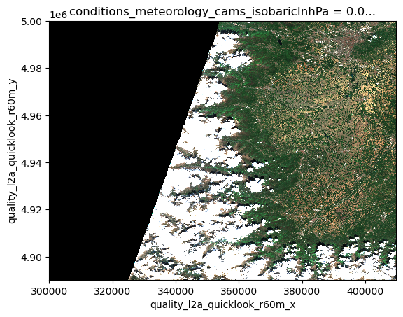
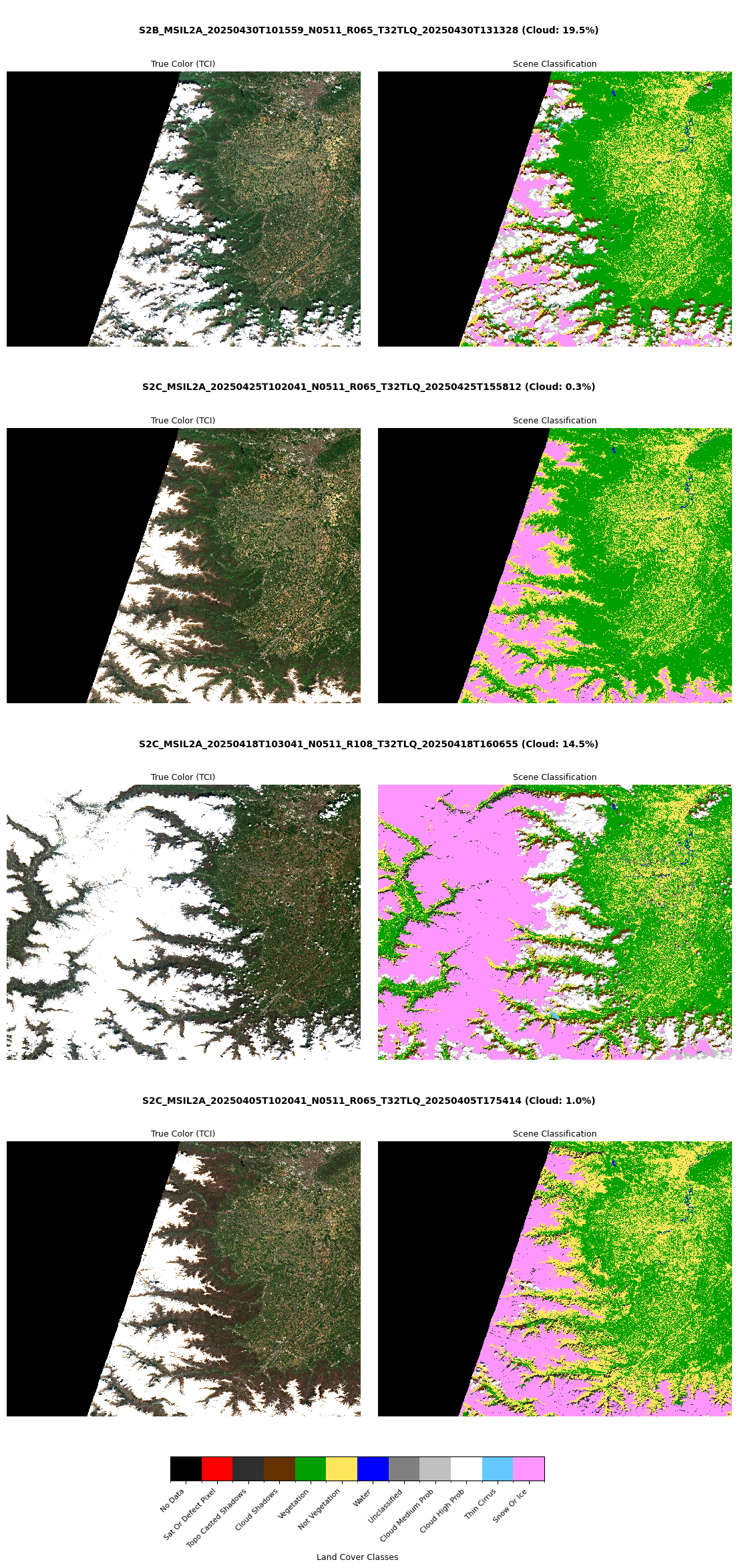
We can view side by side the RGB quicklook and the SCL (Scene Classification Layer) for all the returned STAC Items:
def visualize_items_table(items):
    """
    Visualize multiple Sentinel-2 items with scene IDs centered above each row,
    followed by two columns (RGB and SCL).

    Parameters:
        items (list): List of STAC items
    """
    num_items = len(items)
    row_height = 7  # Approximate height per item
    fig_height = min(row_height * num_items, 24)

    fig = plt.figure(figsize=(14, fig_height))

    # Create height ratios: 0.3 for title row, 1.7 for image row (per item)
    height_ratios = []
    for _ in range(num_items):
        height_ratios.extend([0.3, 1.7])  # first is title, second is images

    gs = GridSpec(
        num_items * 2, 2, height_ratios=height_ratios, hspace=0.1, wspace=0.05
    )

    # Create colorbar axis (positioned below all plots)
    scl_cbar_ax = fig.add_axes([0.3, 0.03, 0.4, 0.015])  # [left, bottom, width, height]

    for i, item in enumerate(items):
        try:
            # Add centered title for the row
            title_ax = fig.add_subplot(gs[i * 2, :])  # Span both columns
            title_text = f"{item.id} (Cloud: {item.properties['eo:cloud_cover']:.1f}%)"
            title_ax.text(
                0.5,
                0.5,
                title_text,
                ha="center",
                va="center",
                fontsize=10,
                fontweight="bold",
            )
            title_ax.axis("off")

            # Load the dataset
            ds = xr.open_dataset(
                item.assets["product"].href,
                **item.assets["product"].extra_fields["xarray:open_datatree_kwargs"],
            )

            # RGB Column
            ax1 = fig.add_subplot(gs[i * 2 + 1, 0])
            try:
                if "quality_l2a_quicklook_r60m_tci" in ds:
                    ds.quality_l2a_quicklook_r60m_tci.plot.imshow(ax=ax1)
                    ax1.set_title("True Color (TCI)", pad=5, fontsize=9)
                else:
                    ax1.text(
                        0.5,
                        0.5,
                        "No RGB quicklook",
                        ha="center",
                        va="center",
                        fontsize=8,
                    )
            except Exception:
                ax1.text(0.5, 0.5, "RGB Error", ha="center", va="center", fontsize=8)
            ax1.axis("off")

            # SCL Column
            ax2 = fig.add_subplot(gs[i * 2 + 1, 1])
            try:
                if "conditions_mask_l2a_classification_r60m_scl" in ds:
                    scl = ds.conditions_mask_l2a_classification_r60m_scl.compute()

                    # Apply classification attributes
                    scl.attrs.update(
                        {
                            "flag_values": [0, 1, 2, 3, 4, 5, 6, 7, 8, 9, 10, 11],
                            "flag_meanings": (
                                "no_data sat_or_defect_pixel topo_casted_shadows cloud_shadows vegetation not_vegetation water unclassified cloud_medium_prob cloud_high_prob thin_cirrus snow_or_ice"
                            ),
                            "flag_colors": (
                                "#000000 #ff0000 #2f2f2f #643200 #00a000 #ffe65a #0000ff #808080 #c0c0c0 #ffffff #64c8ff #ff96ff"
                            ),
                        }
                    )

                    cmap = mcolors.ListedColormap(scl.attrs["flag_colors"].split(" "))
                    norm = mcolors.BoundaryNorm(
                        boundaries=np.arange(13) - 0.5, ncolors=12  # For 12 classes
                    )

                    img_scl = scl.plot.imshow(
                        ax=ax2, cmap=cmap, norm=norm, add_colorbar=False
                    )
                    ax2.set_title("Scene Classification", pad=5, fontsize=9)

                    # Create colorbar once
                    if i == 0:
                        cbar = fig.colorbar(
                            img_scl,
                            cax=scl_cbar_ax,
                            orientation="horizontal",
                            ticks=np.arange(12),
                        )
                        class_labels = [
                            label.replace("_", " ").title()
                            for label in scl.attrs["flag_meanings"].split()
                        ]
                        cbar.ax.set_xticklabels(
                            class_labels, rotation=45, ha="right", fontsize=8
                        )
                        cbar.set_label("Land Cover Classes", fontsize=9)

                else:
                    ax2.text(
                        0.5, 0.5, "No SCL layer", ha="center", va="center", fontsize=8
                    )
            except Exception:
                ax2.text(0.5, 0.5, "SCL Error", ha="center", va="center", fontsize=8)
            ax2.axis("off")

        except Exception as e:
            print(f"Error processing item {item.id}: {str(e)}")
            continue

    plt.tight_layout()
    plt.subplots_adjust(bottom=0.07, top=0.95)  # Adjust for colorbar and titles
    plt.show()


visualize_items_table(items)
/tmp/ipykernel_2583155/2474849155.py:126: UserWarning: This figure includes Axes that are not compatible with tight_layout, so results might be incorrect.
plt.tight_layout()
Sentinel-1 GRD Item Search
Querying Sentinel-1 L1 GRD collection given bounding box, orbit direction and orbit track number.
# Load the STAC catalog
catalog = pystac_client.Client.open("https://stac.core.eopf.eodc.eu")

# Search for Sentinel-1 GRD items matching the metadata characteristics
items = list(
    catalog.search(
        collections=["sentinel-1-l1-grd"],
        bbox=[29.922651, -9.648995, 32.569355, -7.391839],
        datetime=[
            "2025-09-09T00:00:00Z",
            "2025-09-13T23:59:00Z",
        ],
        query={
            "sat:orbit_state": {"eq": "ascending"},
            "sat:relative_orbit": {"eq": 174},
        },
    ).items()
)
items
[<Item id=S1A_IW_GRDH_1SDV_20250913T161934_20250913T161959_060971_079880_E055>,
<Item id=S1A_IW_GRDH_1SDV_20250913T161905_20250913T161934_060971_079880_AB93>]Sentinel-1 GRD Visualization
Opening the first STAC Item and plot the VH polarization
item = items[0]

ds = xr.open_dataset(
    item.assets["product"].href,
    **item.assets["product"].extra_fields["xarray:open_datatree_kwargs"],
    variables="VH_measurements*",
)

plt.imshow(ds["VH_measurements_grd"][::10, ::10].to_numpy(), vmin=0, vmax=200)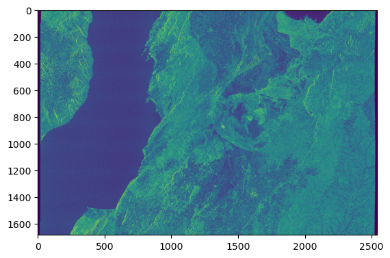
The Sentinel-1 visualization is off due to the EOPF CPM version used for the data conversion. The data must be converted with eopf >= 2.6.1.
print(item.assets["product"].href.split("/cpm_")[1].split("/")[0])v256