Intoduction to the xarray EOPF backend
Access and explore analysis-ready and native EOPF Zarr data using xarray

Run this notebook interactively with all dependencies pre-installed
Introduction
xarray-eopf is a Python package that extends xarray with a custom backend called "eopf-zarr". This backend enables seamless access to ESA EOPF data products stored in the Zarr format, presenting them as analysis-ready data structures.
This notebook demonstrates how to use the xarray-eopf backend to access EOPF Zarr datasets. It highlights the key features currently supported by the backend.
🐙 GitHub: EOPF Sample Service – xarray-eopf
❗ Issue Tracker: Submit or view issues
📘 Documentation: xarray-eopf Docs
Install the xarray-eopf Backend
The backend is implemented as an xarray plugin and can be installed using either pip or conda/mamba from the conda-forge channel.
📦 PyPI: xarray-eopf on PyPI
pip install xarray-eopf🐍 Conda (conda-forge): xarray-eopf on Anaconda
conda install -c conda-forge xarray-eopfYou can also use Mamba as a faster alternative to Conda:
mamba install -c conda-forge xarray-eopf
Import Modules
The xarray-eopf backend is implemented as a plugin for xarray. Once installed, it registers automatically and requires no additional import. You can simply import xarray as usual:
import datetime

import pystac_client
import xarray as xr
Main Features of the xarray-eopf Backend
The xarray-eopf backend for EOPF data products can be selecterd by setting engine="eopf-zarr" in xarray.open_dataset(..) and xarray.open_datatree(..) method. All data access is lazy, meaning that data is only loaded when required—for example, during plotting or when writing to storage. It supports two modes of operation:
Analysis Mode (default)
Native Mode
Native Mode
Represents EOPF products without modification using xarray’s DataTree and Dataset.
open_dataset(path, engine="eopf-zarr", op_mode="native", chunks={})— Returns a flattened version of the data treeopen_datatree(path, engine="eopf-zarr", op_mode="native", chunks={})— Returns the fullDataTree, same asxr.open_datatree(.., engine="zarr")
Analysis Mode
Provides an analysis-ready, resampled view of the data (currently for Sentinel-2 only).
open_dataset(path, engine="eopf-zarr", op_mode="analysis", chunks={})— Loads Sentinel-2 products in a harmonized, analysis-ready formatopen_datatree(path, engine="eopf-zarr", op_mode="analysis", chunks={})— Not implemented in this mode (NotImplementedError)
In the following sections, we demonstrate these functions using a Sentinel-2 L2A product.
For additional examples, refer to the notebooks provided for each Sentinel-1, Sentinel-2, and Sentinel-3 product, available in both native and analysis modes.
The native mode operates identically across all Sentinel missions. In contrast, the analysis mode is customized for each individual mission, as illustrated in the respective notebook examples.
Further information about the analysis mode for each Sentinel mission can be found in the xarray-eopf Guide.
Find a Sentinel Zarr Sample via STAC
To obtain a product URL, you can use the STAC Browser to search for a Sentinel-2 tile. Here, the query parameter is used to select tiles with less than 40% cloud cover, improving the chances of a clear plot.
catalog = pystac_client.Client.open("https://stac.core.eopf.eodc.eu")
items = list(
    catalog.search(
        collections=["sentinel-2-l2a"],
        bbox=[7.2, 44.5, 7.4, 44.7],
        datetime=[str(datetime.date.today() - datetime.timedelta(days=30)), None],
        query={"eo:cloud_cover": {"lt": 40}},
    ).items()
)
items
[<Item id=S2A_MSIL2A_20260326T102701_N0512_R108_T32TLQ_20260326T172711>,
<Item id=S2B_MSIL2A_20260326T102019_N0512_R065_T32TLQ_20260326T155529>,
<Item id=S2B_MSIL2A_20260319T103019_N0512_R108_T32TLQ_20260319T151320>,
<Item id=S2A_MSIL2A_20260316T103041_N0512_R108_T32TLQ_20260316T184508>,
<Item id=S2B_MSIL2A_20260316T101649_N0512_R065_T32TLQ_20260316T155405>,
<Item id=S2A_MSIL2A_20260313T101741_N0512_R065_T32TLQ_20260313T171916>,
<Item id=S2C_MSIL2A_20260304T102921_N0512_R108_T32TLQ_20260304T160811>]Next, we can inspect the item’s contents, including the additional field xarray:open_datatree_kwargs, which provides the arguments needed to open the product using Xarray’s eopf-zarr engine.
item = items[0]
itemOpen Sentinel-2 Level-2A in Native Mode as DataTree
We can use the "product" asset to obtain the href and xarray:open_datatree_kwargs from the STAC item, and open the product as an xarray.DataTree as shown below:
dt = xr.open_datatree(
    item.assets["product"].href,
    **item.assets["product"].extra_fields["xarray:open_datatree_kwargs"]
)
dtAs an example, we plot the red band (b04) at 60 meters resolution, which will trigger loading and visualization of the data.
dt.measurements.reflectance.r60m.b04.plot.imshow(vmin=0, vmax=1)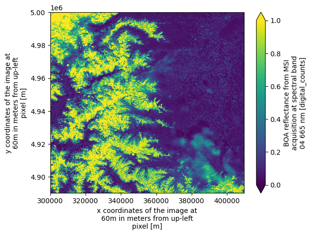
Open Sentinel-2 Level-2A Reflectance Groups in Native Mode as Dataset
Similarly, we can open the individual reflectance groups at 10 m (asset "SR_10m"), 20 m (asset "SR_20m"), and 60 m (asset "SR_60m") to access each group as an xarray.Dataset, as shown below:
ds = xr.open_dataset(
    item.assets["SR_60m"].href,
    **item.assets["SR_60m"].extra_fields["xarray:open_dataset_kwargs"]
)
dsWe can plot an RGB image as an example, using the red (b04), green (b03), and blue (b02) spectral bands.
ax = (
    (ds[["b04", "b03", "b02"]].to_dataarray(dim="band") / 0.3)
    .clip(0, 1)
    .plot.imshow(rgb="band")
)
ax.axes.set_aspect("equal")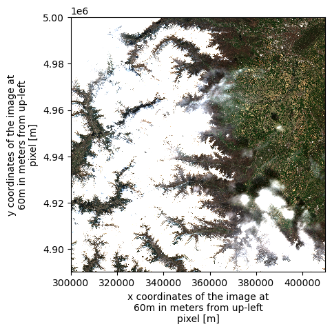
Open Sentinel-2 Level-2A in Native Mode as Dataset
The xarray.DataTree data model is relatively new, introduced in xarray v2024.10.0 (October 2024). To support compatibility with existing workflows that rely on the traditional xr.Dataset model, we provide the function xarray.open_dataset(path, engine="eopf-zarr", op_mode="native", **kwargs). This function flattens the DataTree structure and returns a single xr.Dataset.
In this process, hierarchical groups within the Zarr product are removed by converting their contents into standalone datasets and merging them into one. To ensure uniqueness, variable and dimension names are prefixed with their original group paths, using an underscore (_) as the default separator. For example, a variable named b02 located in the group measurements/reflectance/r10m will be renamed to measurements_reflectance_r10m_b02 in the returned dataset.
ds = xr.open_dataset(
    item.assets["product"].href,
    engine="eopf-zarr",
    op_mode="native",
    chunks={},
)
dsThe separator character used in flattened variable names can be customized via the group_sep parameter. Additionally, you can filter the returned variables using the variables keyword argument, which accepts a string, an iterable of names, or a regular expression (regex) pattern.
ds = xr.open_dataset(
    item.assets["product"].href,
    engine="eopf-zarr",
    op_mode="native",
    chunks={},
    group_sep="/",
    variables="measurements/r60m/b0[234]",
)
dsFollowing the previous steps, we can now select a data variable and display the RGB image as an example.
array = ds[
    ["measurements/r60m/b04", "measurements/r60m/b03", "measurements/r60m/b02"]
].to_dataarray(dim="band")
ax = (array / 0.3).clip(0, 1).plot.imshow(rgb="band")
ax.axes.set_aspect("equal")
Open Sentinel-2 Level-2A in Analysis Mode as Dataset
Next, we use the "product" asset to open the Sentinel-2 product in analysis mode, which presents EOPF products as an analysis-ready xarray Dataset with a single, unified grid mapping. For Sentinel-2, all variables are automatically upscaled or downscaled so that the dataset shares one consistent pair of x and y coordinates. Note that analysis mode is the default in the xarray EOPF plugin.
We use 60 m resolution to keep plotting fast, as full-resolution data can be slow to render in Matplotlib. For full details on xarray.open_dataset configuration options, see the xarray-eopf documentation.
ds = xr.open_dataset(
    items[0].assets["product"].href, engine="eopf-zarr", resolution=60, chunks={}
)
dsAnd we can plot one spectral band as example:
ds.b04.plot(vmin=0, vmax=1)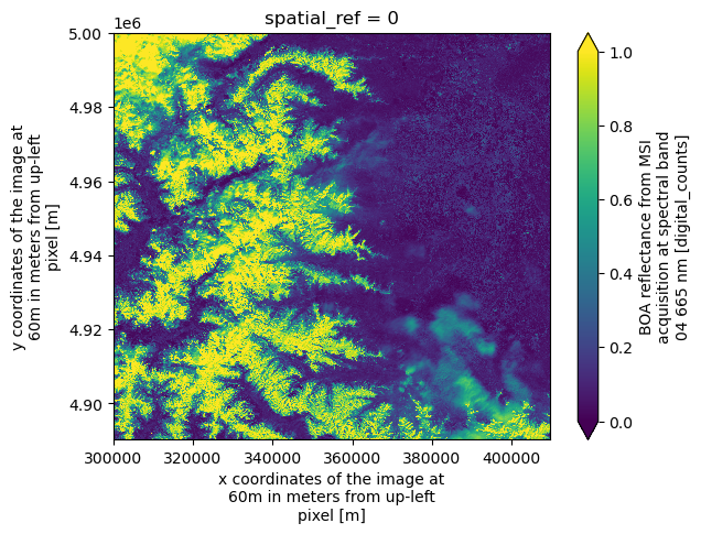
Conclusion
This notebook highlighted the main features of the xarray-eopf backend, which enables seamless access to EOPF Zarr products using familiar Xarray methods (xr.open_dataset and xr.open_datatree) by specifying engine="eopf-zarr". Key takeaways:
Two operation modes:
op_mode="native": Represents EOPF products without modification using Xarray’sDataTreeandDatasetstructures.op_mode="analysis": Provides an analysis-ready, resampled view of the data and is available forxarray.open_datasetonly.
Opening parameters are integrated into the STAC items, allowing streamlined data access and management.
Subgroups of the data tree are resolved via individual STAC assets and can be accessed with
xarray.open_datasetusing the provided parameters.
Future Examples
For additional examples, see the notebooks for Sentinel-1, Sentinel-2, and Sentinel-3 products, in both native and analysis modes.
