xarray EOPF backend - Sentinel-1

Table of Contents¶

Introduction
Import modules
Open a Sentinel-1 GRD
Open a Sentinel-1 Level-2 OCN
Conclusion

Run this notebook interactively with all dependencies pre-installed

Introduction¶

xarray-eopf is a Python package that extends xarray with a custom backend called "eopf-zarr". This backend enables seamless access to ESA EOPF data products stored in the Zarr format, presenting them as analysis-ready data structures.

In this notebook, we demonstrate how to use the xarray-eopf backend to access Sentinel-1 EOPF Zarr products in native mode. All data access is lazy, meaning that data is only loaded when required—for example, during plotting or when writing to storage.

For a general introduction to the xarray EOPF backend, see the introduction notebook.

🐙 GitHub: EOPF Sample Service – xarray-eopf
❗ Issue Tracker: Submit or view issues
📘 Documentation: xarray-eopf Docs

Import Modules¶

The xarray-eopf backend is implemented as a plugin for xarray. Once installed, it registers automatically and requires no additional import. You can simply import xarray as usual:

import datetime

import matplotlib.pyplot as plt
import pystac_client
import xarray as xr

Open a Sentinel-1 GRD¶

We begin with an example that accesses a Sentinel-1 GRD product in native mode.

Find a Sentinel-1 GRD Zarr Sample via STAC¶

To obtain a product URL, you can use the STAC Browser to search for a Sentinel-1 GRD tile.

catalog = pystac_client.Client.open("https://stac.core.eopf.eodc.eu")
items = list(
    catalog.search(
        collections=["sentinel-1-l1-grd"],
        bbox=[7.2, 44.5, 7.4, 44.7],
        datetime=[str(datetime.date.today() - datetime.timedelta(days=30)), None],
    ).items()
)
items

[<Item id=S1C_IW_GRDH_1SDV_20260329T173003_20260329T173028_006982_00E226_9BA1>,
 <Item id=S1A_IW_GRDH_1SDV_20260329T053552_20260329T053617_063838_080734_1F29>,
 <Item id=S1C_IW_GRDH_1SDV_20260328T054254_20260328T054319_006960_00E156_9271>,
 <Item id=S1C_IW_GRDH_1SDV_20260324T172158_20260324T172223_006909_00DF9C_BC61>,
 <Item id=S1A_IW_GRDH_1SDV_20260323T173113_20260323T173138_063758_080437_1B1F>,
 <Item id=S1C_IW_GRDH_1SDV_20260323T053505_20260323T053530_006887_00DED8_A071>,
 <Item id=S1C_IW_GRDH_1SDV_20260323T053440_20260323T053505_006887_00DED8_C5E4>,
 <Item id=S1A_IW_GRDH_1SDV_20260322T054415_20260322T054440_063736_080362_7F26>,
 <Item id=S1A_IW_GRDH_1SDV_20260322T054350_20260322T054415_063736_080362_32F4>,
 <Item id=S1A_IW_GRDH_1SDV_20260318T172306_20260318T172331_063685_080176_BEF4>,
 <Item id=S1C_IW_GRDH_1SDV_20260317T173003_20260317T173028_006807_00DC26_BF98>,
 <Item id=S1A_IW_GRDH_1SDV_20260317T053552_20260317T053617_063663_0800AA_468A>,
 <Item id=S1C_IW_GRDH_1SDV_20260316T054254_20260316T054319_006785_00DB62_1DC1>,
 <Item id=S1C_IW_GRDH_1SDV_20260312T172158_20260312T172223_006734_00D99D_8D64>,
 <Item id=S1A_IW_GRDH_1SDV_20260311T173112_20260311T173137_063583_07FDB1_898F>,
 <Item id=S1C_IW_GRDH_1SDV_20260311T053504_20260311T053529_006712_00D8DB_0DB7>,
 <Item id=S1C_IW_GRDH_1SDV_20260311T053439_20260311T053504_006712_00D8DB_63B6>,
 <Item id=S1A_IW_GRDH_1SDV_20260310T054415_20260310T054440_063561_07FCD9_D8C1>,
 <Item id=S1A_IW_GRDH_1SDV_20260310T054350_20260310T054415_063561_07FCD9_C635>,
 <Item id=S1A_IW_GRDH_1SDV_20260306T172306_20260306T172331_063510_07FAE9_08FD>,
 <Item id=S1C_IW_GRDH_1SDV_20260305T173002_20260305T173027_006632_00D62D_471A>,
 <Item id=S1A_IW_GRDH_1SDV_20260305T053552_20260305T053617_063488_07FA14_B3C9>,
 <Item id=S1C_IW_GRDH_1SDV_20260304T054253_20260304T054318_006610_00D562_2624>,
 <Item id=S1C_IW_GRDH_1SDV_20260228T172157_20260228T172222_006559_00D39F_7632>]

Next, we can inspect the item’s contents, including the additional field xarray:open_datatree_kwargs, which provides the arguments needed to open the product using Xarray’s eopf-zarr engine.

item = items[1]
item

Open Sentinel-1 GRD in native mode as DataTree¶

We can use the "product" asset to obtain the href and xarray:open_datatree_kwargs from the STAC item, and open the product as an xarray.DataTree as shown below:

%%time
dt = xr.open_datatree(
    item.assets["product"].href,
    **item.assets["product"].extra_fields["xarray:open_datatree_kwargs"],
)
dt

CPU times: user 1.96 s, sys: 332 ms, total: 2.29 s
Wall time: 7.32 s

We can extract the `first band as shown below:

ds = dt[dt.groups[1]].measurements.to_dataset()
ds

As an example, we plot the raw GRD array.

ds.grd[::10, ::10].plot(vmax=200, figsize=(13, 8))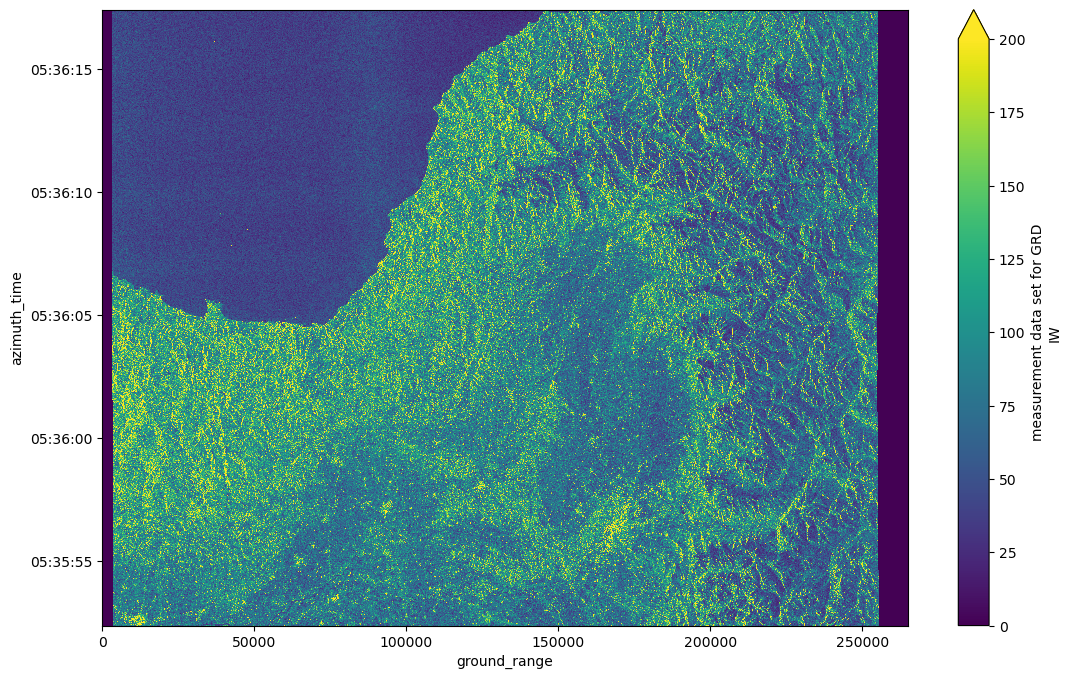

Open Sentinel-1 GRD VH group in native mode as Dataset¶

Similarily, we can open the individual polarisation bands (assets "vh" and "vv") to open the individual groups as an xarray.Dataset as shown below:

%%time
ds = xr.open_dataset(
    item.assets["vh"].href,
    **item.assets["vh"].extra_fields["xarray:open_dataset_kwargs"],
)
ds

CPU times: user 99.2 ms, sys: 23.5 ms, total: 123 ms
Wall time: 1.28 s

Open Sentinel-1 GRD as Dataset¶

The xarray.DataTree model was introduced in xarray v2024.10.0 (October 2024). To maintain compatibility with workflows based on xr.Dataset, the function xarray.open_dataset(..., engine="eopf-zarr", op_mode="native") is provided, which flattens the DataTree into a single dataset.

During this process, hierarchical groups in the Zarr product are merged, and variable as well as dimension names are prefixed with their group paths (using _ by default) to ensure uniqueness. For example, S01SIWGRD_20260316T045550_0025_A364_7C56_080022_VH.measurements becomes S01SIWGRD_20260316T045550_0025_A364_7C56_080022_VH_measurements.

%%time
ds = xr.open_dataset(
    item.assets["product"].href,
    engine="eopf-zarr",
    op_mode="native",
    chunks={},
)
ds

CPU times: user 775 ms, sys: 55.9 ms, total: 831 ms
Wall time: 3.34 s

The separator character used in flattened variable names can be customized via the group_sep parameter. Additionally, you can filter the returned variables using the variables keyword argument, which accepts a string, an iterable of names, or a regular expression (regex) pattern.

In this example, we use a regex to select all arrays associated with the VH band.

ds = xr.open_dataset(
    item.assets["product"].href,
    engine="eopf-zarr",
    op_mode="native",
    chunks={},
    group_sep="/",
    variables="^VH.*",
)
ds

We can now plot the GRD array and the coarse 2d latitude and longitude grids, which can be used for geolocation.

fig, ax = plt.subplots(1, 3, figsize=(15, 4))
ds["VH/measurements/grd"][::10, ::10].plot.imshow(ax=ax[0], vmax=200)
ds["VH/conditions/gcp/longitude"].plot.imshow(ax=ax[1])
ds["VH/conditions/gcp/latitude"].plot.imshow(ax=ax[2])
plt.tight_layout()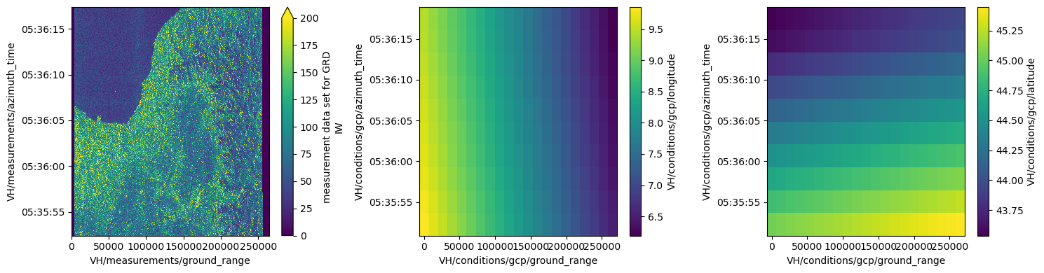

Open a Sentinel-1 Level-2 OCN¶

We now access a Sentinel-1 Level-2 OCN product in native mode. The data access methods shown above apply equally to Sentinel-1 Level-2 OCN products.

Find a Sentinel-1 Level-2 OCN Zarr Sample via STAC¶

To obtain a product URL, you can use the STAC Browser to search for available Sentinel-1 Level-2 OCN tiles.

catalog = pystac_client.Client.open("https://stac.core.eopf.eodc.eu")
items = list(
    catalog.search(
        collections=["sentinel-1-l2-ocn"],
        bbox=[7.2, 44.5, 7.4, 44.7],
        datetime=[str(datetime.date.today() - datetime.timedelta(days=365)), None],
    ).items()
)
items

[<Item id=S1C_IW_OCN__2SDV_20250727T172200_20250727T172225_003409_006DAD_7517>,
 <Item id=S1C_IW_OCN__2SDV_20250726T053506_20250726T053531_003387_006D07_5CDB>,
 <Item id=S1A_IW_OCN__2SDV_20250725T054423_20250725T054448_060236_077C52_B0C4>,
 <Item id=S1C_IW_OCN__2SDV_20250608T053504_20250608T053529_002687_0058C3_0307>,
 <Item id=S1C_IW_OCN__2SDV_20250528T172156_20250528T172221_002534_00545C_B05B>,
 <Item id=S1C_IW_OCN__2SDV_20250527T053503_20250527T053528_002512_0053BB_6400>,
 <Item id=S1A_IW_OCN__2SDV_20250526T054426_20250526T054451_059361_075E24_149E>,
 <Item id=S1C_IW_OCN__2SDV_20250521T173000_20250521T173025_002432_00517D_7E24>,
 <Item id=S1A_IW_OCN__2SDV_20250521T053603_20250521T053628_059288_075B98_AA29>,
 <Item id=S1C_IW_OCN__2SDV_20250516T172154_20250516T172219_002359_004F85_9A03>,
 <Item id=S1C_IW_OCN__2SDV_20250515T053501_20250515T053526_002337_004EE6_9031>,
 <Item id=S1A_IW_OCN__2SDV_20250514T054426_20250514T054451_059186_075813_CC48>,
 <Item id=S1C_IW_OCN__2SDV_20250509T172959_20250509T173024_002257_004CA9_7DE0>,
 <Item id=S1A_IW_OCN__2SDV_20250509T053603_20250509T053628_059113_07558F_D8D2>,
 <Item id=S1C_IW_OCN__2SDV_20250504T172154_20250504T172219_002184_004A3B_37AC>,
 <Item id=S1C_IW_OCN__2SDV_20250503T053500_20250503T053525_002162_004973_C407>,
 <Item id=S1A_IW_OCN__2SDV_20250502T054426_20250502T054451_059011_07519F_AE2A>,
 <Item id=S1C_IW_OCN__2SDV_20250427T172953_20250427T173028_002082_004585_C427>,
 <Item id=S1A_IW_OCN__2SDV_20250427T053604_20250427T053629_058938_074EBB_1370>,
 <Item id=S1C_IW_OCN__2SDV_20250422T172143_20250422T172213_002009_00413B_A45B>,
 <Item id=S1A_IW_OCN__2SDV_20250420T054426_20250420T054451_058836_074A88_32B5>,
 <Item id=S1C_IW_OCN__2SDV_20250415T172952_20250415T173022_001907_003B30_96E8>,
 <Item id=S1A_IW_OCN__2SDV_20250415T053603_20250415T053628_058763_074791_5F66>,
 <Item id=S1C_IW_OCN__2SDV_20250414T054312_20250414T054341_001885_0039D4_FC7B>]

item = items[0]
item

Open Sentinel-1 Level-2 OCN as DataTree¶

We can use the "product" asset to obtain the href and xarray:open_datatree_kwargs from the STAC item, and open the product as an xarray.DataTree as shown below:

%%time
dt = xr.open_datatree(
    item.assets["product"].href,
    **item.assets["product"].extra_fields["xarray:open_datatree_kwargs"],
)
dt

CPU times: user 246 ms, sys: 8.68 ms, total: 255 ms
Wall time: 654 ms

We can extract the ocean wind field dataset as shown below:

ds = dt[dt.owi.groups[1]].measurements.to_dataset()
ds

As an example, we plot the two ocean wind field array.

fig, ax = plt.subplots(1, 2, figsize=(12, 5))
ds.wind_direction.plot(ax=ax[0])
ds.wind_speed.plot(ax=ax[1])
plt.tight_layout()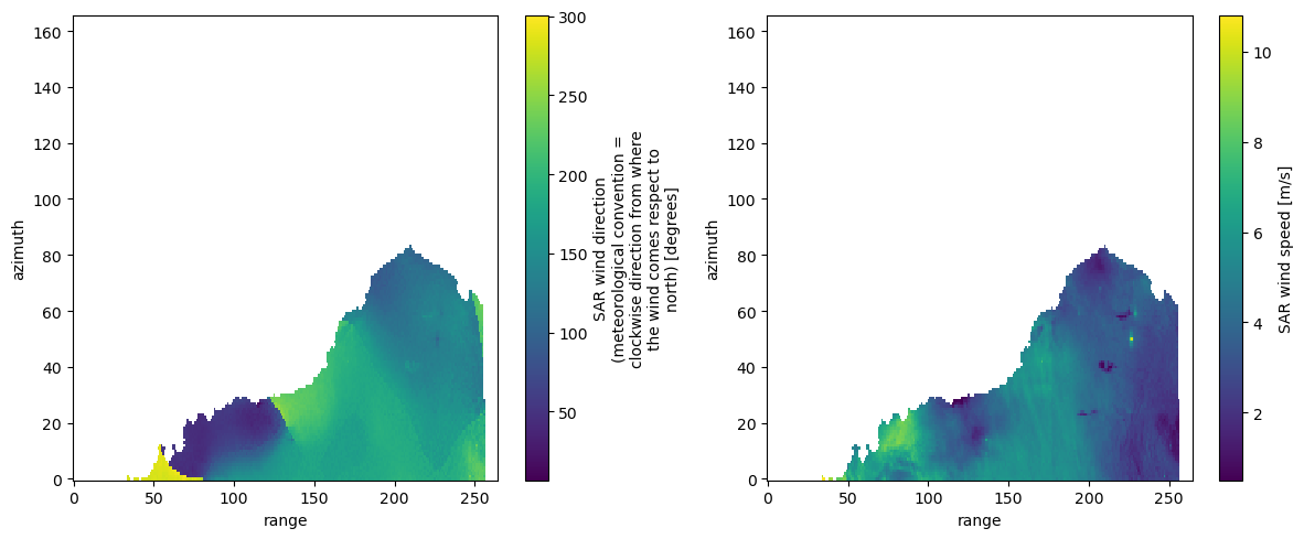

Open Sentinel-1 Level-2 OCN OWI Group as Dataset¶

We can access the individual sub-groups directly by using the assets "osw", "owi", and "rvl". The opening parameters are stored in the asset’s extra field "xarray:open_dataset_kwargs".

ds = xr.open_dataset(
    item.assets["owi"].href,
    **item.assets["owi"].extra_fields["xarray:open_dataset_kwargs"],
)
ds

Conclusion¶

This notebook demonstrates how to access Sentinel-1 EOPF Zarr samples in native mode using the xarray-eopf plugin. Key takeaways are:

Access Sentinel-1 Level-1 GRD, and Sentinel-1 Level-2 OCN products.
Open the full Zarr store as an xr.DataTree using xr.open_datatree and the asset "product".
Open subgroups (e.g., "vh", "vv", "owi", and "rvl") as xr.Dataset using xr.open_dataset.
Open the full Zarr store as a flattened xr.Dataset using xr.open_dataset and the asset "product".
Filter variables using the variables keyword argument.

Note:
This notebook only covers the native mode, which presents the data as close as possible to the original product.
The anaylsis mode will be presented once implemented.
Examples for Sentienl-1 SLC will be presented once updated Zarr samples are published through the STAC API.