xarray EOPF backend - Sentinel-2 Analysis Mode

Table of Contents¶

Introduction
Main Features of the Analysis Mode for Sentinel-2
Import modules
Open a Sentinel-2 Level-1C
Open a Sentinel-2 Level-2A
Conclusion

Run this notebook interactively with all dependencies pre-installed

Introduction¶

xarray-eopf is a Python package that extends xarray with a custom backend called "eopf-zarr". This backend enables seamless access to ESA EOPF data products stored in the Zarr format, presenting them as analysis-ready data structures.

In this notebook, we demonstrate how to use the xarray-eopf backend to access Sentinel-2 EOPF Zarr products in analysis mode. All data access is lazy, meaning that data is only loaded when required—for example, during plotting or when writing to storage.

For a general introduction to the xarray EOPF backend, see the introduction notebook.
For an example of the native mode, see the Sentinel-2 native mode notebook.

🐙 GitHub: EOPF Sample Service – xarray-eopf
❗ Issue Tracker: Submit or view issues
📘 Documentation: xarray-eopf Docs

Main Features of the Analysis Mode for Sentinel-2¶

The analysis mode provides EOPF products as analysis-ready xarray.Dataset objects on a single, unified spatial grid. For Sentinel-2, this means all variables are automatically upscaled or downscaled so that they share a consistent pair of x and y coordinates.

Native resolution of Sentinel-2 spectral bands¶

10 m: B02, B03, B04, B08
20 m: B05, B06, B07, B8A, B11, B12
60 m: B01, B09, B10

Key properties of Sentinel-2 analysis mode¶

Default mode for the "eopf-zarr" backend
Selectable spatial resolution: 10 m (default), 20 m, or 60 m
Automatic resampling to align bands of different resolutions:
- Upsampling via interpolation (default is nearest for integer arrays (e.g. Sentinel-2 L2A SCL, else bilinear),
- Downsampling via aggregation (default is center for integer arrays (e.g. Sentinel-2 L2A SCL, else mean)
Spatial subsetting via the bbox argument
Reprojection to different CRS via the crs argument
Flexible variable selection using names or regex patterns

For full details on opening parameters, see the Analysis Mode documentation and, specifically for Sentinel-2, the Sentinel-2 Analysis Mode guide.

Import Modules¶

The xarray-eopf backend is implemented as a plugin for xarray. Once installed, it registers automatically and requires no additional import. You can simply import xarray as usual:

import datetime

import matplotlib.colors as mcolors
import matplotlib.pyplot as plt
import numpy as np
import pystac_client
import xarray as xr

Open a Sentinel-2 Level-1C product¶

We begin with an example that accesses a Sentinel-2 Level-1C product in analysis mode.

Find a Sentinel-2 Level-1C Zarr Sample via STAC¶

To obtain a product URL, you can use the STAC Browser to search for a Sentinel-2 Level-1C tile. Here, the query parameter is used to select tiles with less than 40% cloud cover, improving the chances of a clear plot.

catalog = pystac_client.Client.open("https://stac.core.eopf.eodc.eu")
items = list(
    catalog.search(
        collections=["sentinel-2-l1c"],
        bbox=[7.2, 44.5, 7.4, 44.7],
        datetime=[str(datetime.date.today() - datetime.timedelta(days=30)), None],
        query={"eo:cloud_cover": {"lt": 40}},
    ).items()
)
items

[<Item id=S2A_MSIL1C_20260326T102701_N0512_R108_T32TLQ_20260326T154418>,
 <Item id=S2C_MSIL1C_20260321T101721_N0512_R065_T32TLQ_20260321T143127>,
 <Item id=S2B_MSIL1C_20260319T103019_N0512_R108_T32TLQ_20260319T145744>,
 <Item id=S2A_MSIL1C_20260316T103041_N0512_R108_T32TLQ_20260316T172545>,
 <Item id=S2B_MSIL1C_20260316T101649_N0512_R065_T32TLQ_20260316T153332>,
 <Item id=S2A_MSIL1C_20260313T101741_N0512_R065_T32TLQ_20260313T153853>,
 <Item id=S2C_MSIL1C_20260304T102921_N0512_R108_T32TLQ_20260304T140806>]

item = items[0]

Open Sentinel-2 Level-1C with default parameters¶

We can now open the Sentinel-2 product in analysis mode. Since this is the default, the op_mode parameter does not need to be specified.

The following cell returns a lazy dataset, with all bands resampled to 60 m resolution. This lower resolution is chosen to keep plotting fast, as rendering full-resolution data in Matplotlib can be slow.

ds = xr.open_dataset(
    item.assets["product"].href, engine="eopf-zarr", resolution=60, chunks={}
)
ds

As an example, we plot the red band (b04), which triggers the loading and visualization of the data. Note that the red band is only available at 10 m resolution in the Level-1C product. Therefore, when plotting, the array is first loaded at 10 m resolution and then aggregated before being displayed, which may take some time.

ds.b04.plot(vmin=0.0, vmax=1.0)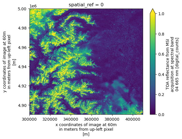

Spatial Resampling, Subsetting and Reprojection¶

We can also change the resolution and display only a subset of the data by specifying the bbox argument, as shown below.

ds = xr.open_dataset(
    item.assets["product"].href,
    engine="eopf-zarr",
    resolution=10,
    bbox=[340000, 4900000, 360000, 4920000],
    chunks={},
)
ds

As an example, we plot again the red band (b04).

ds.b04.plot(vmin=0.0, vmax=1.0)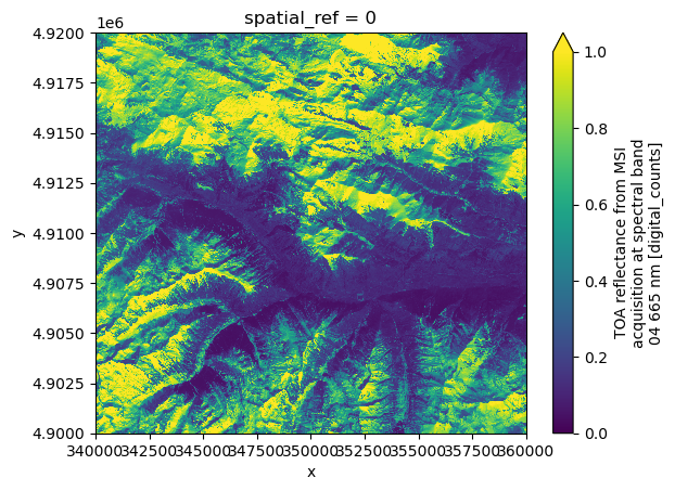

We can request the same area in WGS84 geographic coordinates by specifying crs="EPSG:4326". Note that both the resolution and bbox must be provided in the CRS units (i.e., degrees).

ds = xr.open_dataset(
    item.assets["product"].href,
    engine="eopf-zarr",
    resolution=0.0002,
    crs="EPSG:4326",
    bbox=[7.0, 44.2, 7.3, 44.4],
    chunks={},
)
ds

For comparison, we plot the red band (b04).

ds.b04.plot(vmin=0.0, vmax=1.0)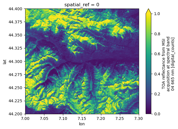

Explore Different Aggregation Methods¶

As mentioned above, the default aggregation method for spectral bands during downsampling is to take the mean of each superpixel. We can also specify the aggregation method via the keyword argument agg_methods, which will be demonstrated in the next cell.

Note: The interpolation method can also be specified when upsampling via the keyword argument interp_methods. Both keywords can be also a mapping from varaible name or data type to resampling method. More details are available in the Analysis Mode documentation.

ds_agg_max = xr.open_dataset(
    item.assets["product"].href,
    engine="eopf-zarr",
    chunks={},
    resolution=60,
    agg_methods="max",
)
ds_agg_mean = xr.open_dataset(
    item.assets["product"].href, engine="eopf-zarr", chunks={}, resolution=60
)

fig, ax = plt.subplots(1, 3, figsize=(18, 5))
ds_agg_max.b04[1500:, 1500:].plot(ax=ax[0], vmin=0.0, vmax=0.6)
ax[0].set_title("Aggregation method 'max'")
ds_agg_mean.b04[1500:, 1500:].plot(ax=ax[1], vmin=0.0, vmax=0.6)
ax[1].set_title("Aggregation method 'mean'")
(ds_agg_max.b04 - ds_agg_mean.b04)[1500:, 1500:].plot(
    ax=ax[2], vmin=-0.1, vmax=0.1, cmap="bwr"
)
ax[2].set_title("Difference")
plt.tight_layout()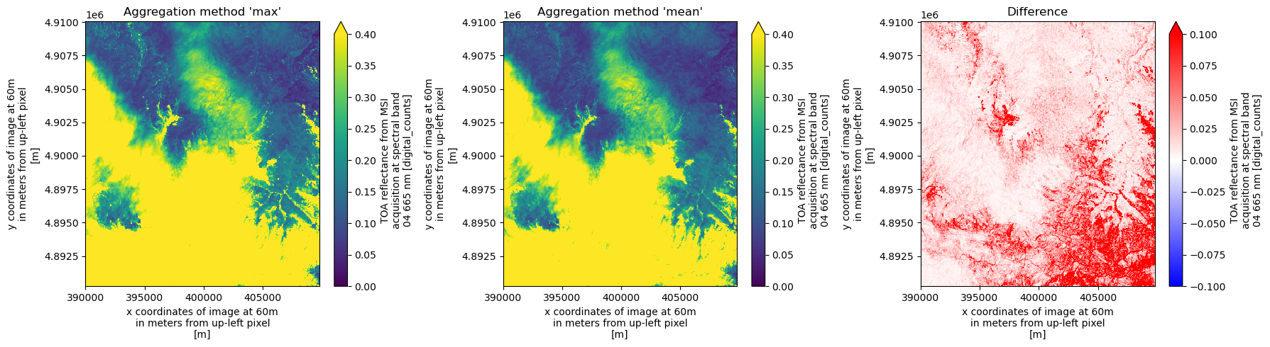

Support for Common Band Names¶

Support has been added for common band names from the STAC EO extension in Sentinel-2 analysis mode.

The variables parameter now accepts standard spectral names such as blue, green, red, nir, and others.

The next cell demonstrates an example where we filter spectral bands using these common names.

ds = xr.open_dataset(
    item.assets["product"].href,
    engine="eopf-zarr",
    chunks={},
    resolution=60,
    variables=["red", "green", "blue", "nir"],
)
ds

ds.red.plot(vmin=0.0, vmax=1.0)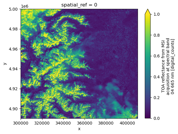

Open Sentinel-2 Level-2A product¶

Find a Sentinel-2 Level-2A Zarr Sample via STAC¶

To obtain a product URL, you can use the STAC Browser to search for available Sentinel-2 Level-2A tiles. Also here, the query parameter is used to select tiles with less than 40% cloud cover, improving the chances of a clear plot.

catalog = pystac_client.Client.open("https://stac.core.eopf.eodc.eu")
items = list(
    catalog.search(
        collections=["sentinel-2-l2a"],
        bbox=[7.2, 44.5, 7.4, 44.7],
        datetime=[str(datetime.date.today() - datetime.timedelta(days=30)), None],
        query={"eo:cloud_cover": {"lt": 40}},
    ).items()
)
items

[<Item id=S2A_MSIL2A_20260326T102701_N0512_R108_T32TLQ_20260326T172711>,
 <Item id=S2B_MSIL2A_20260326T102019_N0512_R065_T32TLQ_20260326T155529>,
 <Item id=S2B_MSIL2A_20260319T103019_N0512_R108_T32TLQ_20260319T151320>,
 <Item id=S2A_MSIL2A_20260316T103041_N0512_R108_T32TLQ_20260316T184508>,
 <Item id=S2B_MSIL2A_20260316T101649_N0512_R065_T32TLQ_20260316T155405>,
 <Item id=S2A_MSIL2A_20260313T101741_N0512_R065_T32TLQ_20260313T171916>,
 <Item id=S2C_MSIL2A_20260304T102921_N0512_R108_T32TLQ_20260304T160811>]

item = items[0]

ds = xr.open_dataset(
    item.assets["product"].href,
    engine="eopf-zarr",
    chunks={},
    resolution=60,
)
ds

Open Sentinel-2 Level-2A with default parameters¶

We can now open the Sentinel-2 product in analysis mode.

Also here, the following cell returns a lazy dataset, with all bands resampled to 60 m resolution. This lower resolution is chosen to keep plotting fast, as above.

For the SCL variable, the flag names, values, and corresponding colors are stored in the attributes to simplify visualization. The colors follow the Sentinel Hub specifications.

In the next cell, we use these flag values and names to plot the categorical SCL dataset.

fig, ax = plt.subplots(1, 2, figsize=(12, 5))

ds.b04.plot(ax=ax[0], vmin=0.0, vmax=0.3)
ax[0].set_title("B04 - red")

cmap = mcolors.ListedColormap(ds.scl.attrs["flag_colors"].split(" "))
nb_colors = len(ds.scl.attrs["flag_values"])
norm = mcolors.BoundaryNorm(
    boundaries=np.arange(nb_colors + 1) - 0.5, ncolors=nb_colors
)
im = ds.scl.plot.imshow(ax=ax[1], cmap=cmap, norm=norm, add_colorbar=False)
cbar = fig.colorbar(im, ax=ax[1], ticks=ds.scl.attrs["flag_values"])
cbar.ax.set_yticklabels(ds.scl.attrs["flag_meanings"].split(" "))
cbar.set_label("Class")
ax[1].set_title("Scene classification layer")

plt.tight_layout()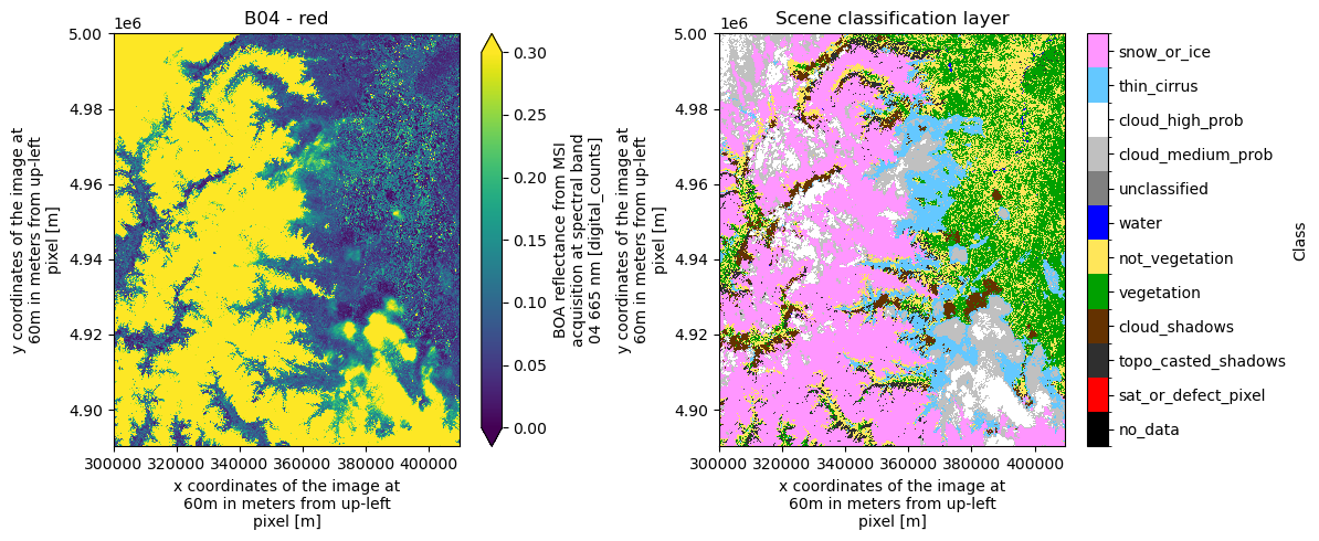

Conclusion¶

This notebook demonstrates how to access Sentinel-2 EOPF Zarr samples in analysis mode using the xarray-eopf plugin. The key takeaways are:

Analysis mode is the default op_mode.
In analysis mode, Sentinel-2 variables are automatically resampled (upscaled or downscaled) to share a consistent set of x and y coordinates.
Data can be accessed lazily at a user-defined resolution, bounding box, and CRS, enabling flexible resampling, subsetting, and reprojection.
Common band names defined by the STAC EO extension are supported for variable selection.
Aggregation and interpolation methods can be customized by the user for both downsampling and upsampling.
Scene Classification Layer (SCL) attributes include flag values, meanings, and colors, which can be used directly for visualization.

Note: This notebook only covers analysis mode for Sentinel-2. To learn more about native mode, see the Sentinel-2 native mode notebook.