xarray EOPF backend - Sentinel-2 Native mode

Table of Contents¶

Introduction
Import modules
Open a Sentinel-2 Level-1C
Open a Sentinel-2 Level-2A
Conclusion

Run this notebook interactively with all dependencies pre-installed

Introduction¶

xarray-eopf is a Python package that extends xarray with a custom backend called "eopf-zarr". This backend enables seamless access to ESA EOPF data products stored in the Zarr format, presenting them as analysis-ready data structures.

In this notebook, we demonstrate how to use the xarray-eopf backend to access Sentinel-2 EOPF Zarr products in native mode. All data access is lazy, meaning that data is only loaded when required—for example, during plotting or when writing to storage.

For a general introduction to the xarray EOPF backend, see the introduction notebook.

🐙 GitHub: EOPF Sample Service – xarray-eopf
❗ Issue Tracker: Submit or view issues
📘 Documentation: xarray-eopf Docs

Import Modules¶

The xarray-eopf backend is implemented as a plugin for xarray. Once installed, it registers automatically and requires no additional import. You can simply import xarray as usual:

import datetime

import matplotlib.pyplot as plt
import pystac_client
import xarray as xr

Open a Sentinel-2 Level-1C¶

We begin with an example that accesses a Sentinel-2 Level-1C product in native mode.

Find a Sentinel-2 Level-1C Zarr Sample via STAC¶

To obtain a product URL, you can use the STAC Browser to search for a Sentinel-2 Level-1C tile. Here, the query parameter is used to select tiles with less than 40% cloud cover, improving the chances of a clear plot.

catalog = pystac_client.Client.open("https://stac.core.eopf.eodc.eu")
items = list(
    catalog.search(
        collections=["sentinel-2-l1c"],
        bbox=[7.2, 44.5, 7.4, 44.7],
        datetime=[str(datetime.date.today() - datetime.timedelta(days=30)), None],
        query={"eo:cloud_cover": {"lt": 40}},
    ).items()
)
items

[<Item id=S2A_MSIL1C_20260326T102701_N0512_R108_T32TLQ_20260326T154418>,
 <Item id=S2C_MSIL1C_20260321T101721_N0512_R065_T32TLQ_20260321T143127>,
 <Item id=S2B_MSIL1C_20260319T103019_N0512_R108_T32TLQ_20260319T145744>,
 <Item id=S2A_MSIL1C_20260316T103041_N0512_R108_T32TLQ_20260316T172545>,
 <Item id=S2B_MSIL1C_20260316T101649_N0512_R065_T32TLQ_20260316T153332>,
 <Item id=S2A_MSIL1C_20260313T101741_N0512_R065_T32TLQ_20260313T153853>,
 <Item id=S2C_MSIL1C_20260304T102921_N0512_R108_T32TLQ_20260304T140806>]

Next, we can inspect the item’s contents. The asset "product" links to the entire Zarr store. The additional field xarray:open_datatree_kwargs has been included in the asset "product", which provides the arguments needed to open the product using Xarray’s eopf-zarr engine.

item = items[0]
item

Open Sentinel-2 Level-1C as `xarray.DataTree`¶

We can use the "product" asset to obtain the href and xarray:open_datatree_kwargs from the STAC item, and open the product as an xarray.DataTree as shown below:

dt = xr.open_datatree(
    item.assets["product"].href,
    **item.assets["product"].extra_fields["xarray:open_datatree_kwargs"],
)
dt

As an example, we plot the spectral band 9 (b09) at 60 meters resolution, which will trigger loading and visualization of the data. Additionally, we will plot the viewing and solar zenith angle on the side.

fig, ax = plt.subplots(1, 3, figsize=(15, 5))
dt.measurements.reflectance.r60m.b09.plot.imshow(ax=ax[0], vmin=0, vmax=0.5)
dt.conditions.geometry.sun_angles.sel(angle="zenith").plot.imshow(ax=ax[1])
dt.conditions.geometry.viewing_incidence_angles.sel(angle="zenith", band="b09").mean(
    dim="detector"
).plot.imshow(ax=ax[2])
plt.tight_layout()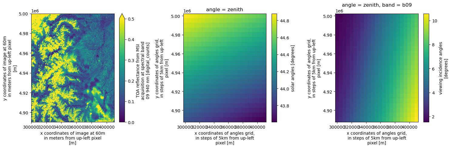

Open Sentinel-2 Level-1C Reflectance Groups as `xarray.Dataset`¶

Similarly, we can open the individual reflectance groups at 10 m (SR_10m), 20 m (SR_20m), and 60 m (SR_60m) resolution as xarray.Dataset objects.

The opening parameters are stored in the asset’s extra field "xarray:open_dataset_kwargs". Note that when opening a group, only the bands available at that resolution (e.g., 10 m) are included.

ds = xr.open_dataset(
    item.assets["SR_10m"].href,
    **item.assets["SR_10m"].extra_fields["xarray:open_dataset_kwargs"],
)
ds

We can also filter the varaibles by band names as shown below:

ds = xr.open_dataset(
    item.assets["SR_10m"].href,
    **item.assets["SR_10m"].extra_fields["xarray:open_dataset_kwargs"],
    variables="b0[234]",
)
ds

And we can plot a cutout of the RGB image, which triggers loading the data.

array = ds[["b04", "b03", "b02"]].to_dataarray(dim="band")
array = array.isel(x=slice(-1830, None), y=slice(-1830, None))
array

ax = (array / 0.3).clip(0, 1).plot.imshow(rgb="band")
ax.axes.set_aspect("equal")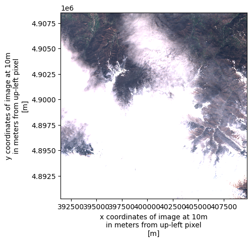

Open Sentinel-2 Level-1C as `xarray.Dataset`¶

The xarray.DataTree model was introduced in xarray v2024.10.0 (October 2024). To maintain compatibility with workflows based on xr.Dataset, the function xarray.open_dataset(..., engine="eopf-zarr", op_mode="native") is provided, which flattens the DataTree into a single dataset.

During this process, hierarchical groups in the Zarr product are merged, and variable as well as dimension names are prefixed with their group paths (using _ by default) to ensure uniqueness. For example, measurements/reflectance/r10m/b02 becomes measurements_reflectance_r10m_b02.

ds = xr.open_dataset(
    item.assets["product"].href,
    engine="eopf-zarr",
    op_mode="native",
    chunks={},
)
ds

The separator character used in flattened variable names can be customized via the group_sep parameter. Additionally, you can filter the returned variables using the variables keyword argument, which accepts a string, an iterable of names, or a regular expression (regex) pattern.

ds = xr.open_dataset(
    item.assets["product"].href,
    engine="eopf-zarr",
    op_mode="native",
    chunks={},
    group_sep="/",
    variables=["measurements/r60m/b09", "measurements/r60m/b10"],
)
ds

Also here, we can plot one spectral band as an example.

ds["measurements/r60m/b09"].plot(vmin=0.0, vmax=1.0)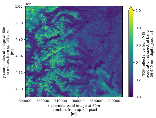

Open a Sentinel-2 Level-2A¶

We now access a Sentinel-2 Level-2A product in native mode. The data access methods shown above apply equally to Level-2A products.

Find a Sentinel-2 Level-2A Zarr Sample via STAC¶

To obtain a product URL, you can use the STAC Browser to search for available Sentinel-2 Level-2A tiles. Also here, the query parameter is used to select tiles with less than 40% cloud cover, improving the chances of a clear plot.

catalog = pystac_client.Client.open("https://stac.core.eopf.eodc.eu")
items = list(
    catalog.search(
        collections=["sentinel-2-l2a"],
        bbox=[7.2, 44.5, 7.4, 44.7],
        datetime=[str(datetime.date.today() - datetime.timedelta(days=30)), None],
        query={"eo:cloud_cover": {"lt": 40}},
    ).items()
)
items

[<Item id=S2A_MSIL2A_20260326T102701_N0512_R108_T32TLQ_20260326T172711>,
 <Item id=S2B_MSIL2A_20260326T102019_N0512_R065_T32TLQ_20260326T155529>,
 <Item id=S2B_MSIL2A_20260319T103019_N0512_R108_T32TLQ_20260319T151320>,
 <Item id=S2A_MSIL2A_20260316T103041_N0512_R108_T32TLQ_20260316T184508>,
 <Item id=S2B_MSIL2A_20260316T101649_N0512_R065_T32TLQ_20260316T155405>,
 <Item id=S2A_MSIL2A_20260313T101741_N0512_R065_T32TLQ_20260313T171916>,
 <Item id=S2C_MSIL2A_20260304T102921_N0512_R108_T32TLQ_20260304T160811>]

item = items[0]
item

Open Sentinel-2 Level-2A as `xarray.DataTree`¶

We can use the "product" asset to obtain the href and xarray:open_datatree_kwargs from the STAC item, and open the product as an xarray.DataTree as shown below:

dt = xr.open_datatree(
    item.assets["product"].href,
    **item.assets["product"].extra_fields["xarray:open_datatree_kwargs"],
)
dt

We can plot the RGB image, the SCL (Scene Classification Layer), the AOT (Aerosol Optical Thickness) map, and the WVP (Water Vapor Content) map at 60 m resolution.

fig, ax = plt.subplots(1, 4, figsize=(20, 5))
dt.measurements.reflectance.r60m.b04.plot.imshow(ax=ax[0], vmin=0.0, vmax=1.0)
dt.conditions.mask.l2a_classification.r60m.scl.plot.imshow(ax=ax[1])
dt.quality.atmosphere.r60m.aot.plot.imshow(ax=ax[2])
dt.quality.atmosphere.r60m.wvp.plot.imshow(ax=ax[3])
plt.tight_layout()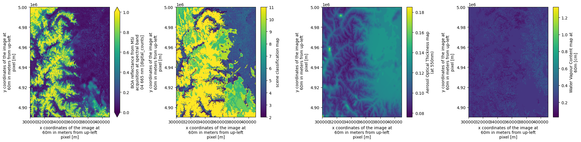

Open Sentinel-2 Level-2A Reflectance Groups as `xarray.Dataset`¶

Similarly, we can open the individual reflectance groups at 10 m (SR_10m), 20 m (SR_20m), and 60 m (SR_60m) resolution as xarray.Dataset objects.

The opening parameters are stored in the asset’s extra field "xarray:open_dataset_kwargs". Note that in Level-2A, some of the native bands are resampled to coarser resoltion. This is idendical to the previous SAFE format.

ds = xr.open_dataset(
    item.assets["SR_60m"].href,
    **item.assets["SR_60m"].extra_fields["xarray:open_dataset_kwargs"],
)
ds

All other data access methods shown for Sentinel Level-1C products apply equally to Level-2A products.

Conclusion¶

This notebook demonstrates how to access Sentinel-2 EOPF Zarr samples in native mode using the xarray-eopf plugin. Key takeaways are:

Access Sentinel-2 Level-1C and Level-2A products.
Open the full Zarr store as an xr.DataTree using xr.open_dataset and the asset "product".
Open subgroups (e.g., spectral reflectance at 10 m, 20 m, or 60 m) as xr.Dataset using xr.open_dataset.
Open the full Zarr store as a flattened xr.Dataset using xr.open_dataset and the asset "product".
Filter variables using the variables keyword argument.
Opening parameters are integrated in STAC assets.

Note: This notebook only covers the native mode, which presents the data as close as possible to the original product.
For an analysis-ready view, see the Sentinel-2 analysis mode notebook.