xarray EOPF backend - Sentinel-3 Analysis Mode
Learn how to access Sentinel-3 products in analysis mode

Table of Contents
Run this notebook interactively with all dependencies pre-installed
Introduction
xarray-eopf is a Python package that extends xarray with a custom backend called "eopf-zarr". This backend enables seamless access to ESA EOPF data products stored in the Zarr format, presenting them as analysis-ready data structures.
In this notebook, we demonstrate how to use the xarray-eopf backend to access Sentinel-3 EOPF Zarr products in analysis mode. All data access is lazy, meaning that data is only loaded when required—for example, during plotting or when writing to storage.
For a general introduction to the xarray EOPF backend, see the introduction notebook.
For an example of the native mode, see the Sentinel-3 native mode notebook.
🐙 GitHub: EOPF Sample Service – xarray-eopf
❗ Issue Tracker: Submit or view issues
📘 Documentation: xarray-eopf Docs
Main Features of the Analysis Mode for Sentinel-3
Sentinel-3 products are provided on their native grid, where each pixel is defined by a latitude/longitude pair, forming a 2D curvilinear (irregular) grid.
The analysis mode applies the rectification algorithm in xcube-resampling to transform this irregular grid into a regular (rectilinear) grid with 1D latitude and longitude coordinates.
For SLSTR products, an additional terrain correction is applied during this process. This is necessary because the original geolocation accounts for Earth curvature, but not for terrain-induced variability due to topography. See the SLSTR product description for details.
For OLCI products, no additional terrain correction is required, as it is already included in the Level-1 data. See the OLCI Level-1 product description for details.
Key Properties of Sentinel-3 Analysis Mode
Default mode for the
"eopf-zarr"backendRectification: converts the 2D curvilinear grid into a rectilinear grid
Spatial subsetting via the
bboxargumentReprojection to different CRS via the
crsargument (default: WGS84, EPSG:4326)Flexible variable selection using names or regular expressions
For full details on available parameters, see the Analysis Mode documentation and, specifically for Sentinel-3, the Sentinel-3 Analysis Mode guide.
Import Modules
The xarray-eopf backend is implemented as a plugin for xarray. Once installed, it registers automatically and requires no additional import. You can simply import xarray as usual:
import datetime

import matplotlib.pyplot as plt
import pyproj
import pystac_client
import xarray as xr
Open a Sentinel-3 OLCI L1 EFR
We begin with an example that accesses a Sentinel-3 OLCI L1 EFR product in analysis mode.
Find a Sentinel-3 OLCI L1 EFR Zarr Sample via STAC
To obtain a product URL, you can use the STAC Browser to search for a Sentinel-3 OLCI Level-1 EFR tile.
catalog = pystac_client.Client.open("https://stac.core.eopf.eodc.eu")
items = list(
    catalog.search(
        collections=["sentinel-3-olci-l1-efr"],
        bbox=[7.2, 44.5, 7.4, 44.7],
        datetime=[str(datetime.date.today() - datetime.timedelta(days=5)), None],
    ).items()
)
items
[<Item id=S3A_OL_1_EFR____20260331T093213_20260331T093513_20260331T113111_0179_137_364_2160_PS1_O_NR_004>,
<Item id=S3A_OL_1_EFR____20260330T095824_20260330T100124_20260330T115813_0179_137_350_2160_PS1_O_NR_004>,
<Item id=S3A_OL_1_EFR____20260330T095824_20260330T100124_20260331T110815_0179_137_350_2160_PS1_O_NT_004>,
<Item id=S3B_OL_1_EFR____20260330T091943_20260330T092243_20260330T112427_0179_118_207_2160_ESA_O_NR_004>,
<Item id=S3B_OL_1_EFR____20260330T091943_20260330T092243_20260331T102059_0179_118_207_2160_ESA_O_NT_004>,
<Item id=S3B_OL_1_EFR____20260329T094553_20260329T094853_20260329T114455_0179_118_193_2160_ESA_O_NR_004>,
<Item id=S3B_OL_1_EFR____20260329T094553_20260329T094853_20260330T110844_0179_118_193_2160_ESA_O_NT_004>,
<Item id=S3B_OL_1_EFR____20260328T101204_20260328T101504_20260328T121637_0179_118_179_2160_ESA_O_NR_004>,
<Item id=S3B_OL_1_EFR____20260328T101204_20260328T101504_20260329T100706_0180_118_179_2160_ESA_O_NT_004>,
<Item id=S3A_OL_1_EFR____20260327T093557_20260327T093857_20260328T103721_0179_137_307_2160_PS1_O_NT_004>,
<Item id=S3A_OL_1_EFR____20260327T093557_20260327T093857_20260327T113653_0180_137_307_2160_PS1_O_NR_004>,
<Item id=S3A_OL_1_EFR____20260326T100207_20260326T100507_20260327T110434_0180_137_293_2160_PS1_O_NT_004>,
<Item id=S3A_OL_1_EFR____20260326T100207_20260326T100507_20260326T120302_0179_137_293_2160_PS1_O_NR_004>,
<Item id=S3B_OL_1_EFR____20260326T092326_20260326T092626_20260327T093749_0179_118_150_2160_ESA_O_NT_004>,
<Item id=S3B_OL_1_EFR____20260326T092326_20260326T092626_20260326T113241_0179_118_150_2160_ESA_O_NR_004>]item = items[0]
itemOpen Sentinel-3 OLCI L1 EFR with default parameters
We can now open the Sentinel-3 product in analysis mode using the xr.open_dataset method. Since this is the default, the op_mode parameter does not need to be specified.
The following cell returns a lazy dataset, with all bands recifified to a regular grid. If no resolution is given, the spatial resolution is estimated from the 2D latitude and longitude grids.
ds = xr.open_dataset(item.assets["product"].href, engine="eopf-zarr", chunks={})
dsAs an example, we plot the red band (oa08_radiance), which triggers data loading, rectification, and visualization of the rectified result.
Note: To speed up rendering of large datasets in Matplotlib, we plot the data at a lower resolution (every 4th pixel).
ds.oa08_radiance[1000:2000, 1000:2000].plot(vmin=0.0, vmax=200.0)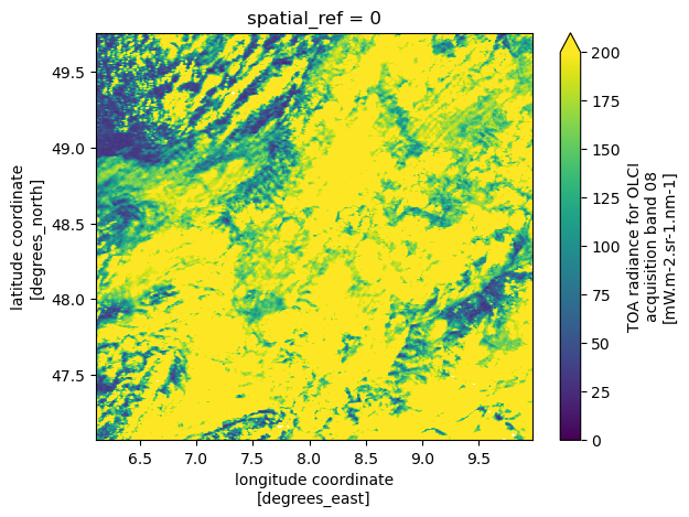
Spatial Resampling, Subsetting and Reprojection
We can also change the resolution and display only a subset of the data by specifying the bbox argument, as shown below.
ds = xr.open_dataset(
    item.assets["product"].href,
    engine="eopf-zarr",
    resolution=0.01,
    bbox=[5, 40, 15, 48],
    chunks={},
)
dsAs an example, we plot again the red band (oa08_radiance).
ds.oa08_radiance.plot(vmin=0.0, vmax=200.0)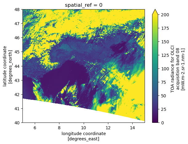
We can request the same area in LAEA CRS by specifying crs="EPSG:3035". Note that both the resolution and bbox must be provided in the CRS units.
bbox = [5, 40, 15, 48]
transformer = pyproj.Transformer.from_crs("EPSG:4326", "EPSG:3035", always_xy=True)
bbox_crs = transformer.transform_bounds(*bbox)
ds = xr.open_dataset(
    item.assets["product"].href,
    engine="eopf-zarr",
    crs="EPSG:3035",
    resolution=1000,
    bbox=bbox_crs,
    chunks={},
)
dsWe plot the red band (oa08_radiance).
ds.oa08_radiance.plot(vmin=0.0, vmax=200.0)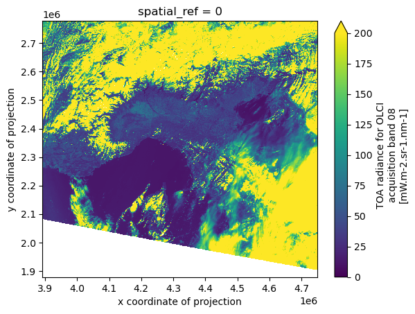
Open a Sentinel-3 OLCI L1 ERR
We now access a Sentinel-3 OLCI L1 ERR product in analysis mode. The data access methods shown above apply equally to Sentinel-3 OLCI L1 EFR.
Find a Sentinel-3 OLCI L1 ERR Zarr Sample via STAC
To obtain a product URL, you can use the STAC Browser to search for available Sentinel-3 OLCI L1 ERR tiles.
catalog = pystac_client.Client.open("https://stac.core.eopf.eodc.eu")
items = list(
    catalog.search(
        collections=["sentinel-3-olci-l1-err"],
        bbox=[7.2, 44.5, 7.4, 44.7],
        datetime=[str(datetime.date.today() - datetime.timedelta(days=5)), None],
    ).items()
)
items
[<Item id=S3A_OL_1_ERR____20260331T092148_20260331T100553_20260331T113030_2645_137_364______PS1_O_NR_004>,
<Item id=S3A_OL_1_ERR____20260330T094806_20260330T103211_20260331T105708_2645_137_350______PS1_O_NT_004>,
<Item id=S3A_OL_1_ERR____20260330T094806_20260330T103211_20260330T115732_2645_137_350______PS1_O_NR_004>,
<Item id=S3B_OL_1_ERR____20260330T090925_20260330T095330_20260331T100829_2645_118_207______ESA_O_NT_004>,
<Item id=S3B_OL_1_ERR____20260330T090925_20260330T095330_20260330T113721_2645_118_207______ESA_O_NR_004>,
<Item id=S3B_OL_1_ERR____20260329T093543_20260329T101948_20260330T105135_2645_118_193______ESA_O_NT_004>,
<Item id=S3B_OL_1_ERR____20260329T093543_20260329T101948_20260329T120344_2645_118_193______ESA_O_NR_004>,
<Item id=S3B_OL_1_ERR____20260328T100201_20260328T104605_20260329T095351_2644_118_179______ESA_O_NT_004>,
<Item id=S3B_OL_1_ERR____20260328T100201_20260328T104605_20260328T122605_2644_118_179______ESA_O_NR_004>,
<Item id=S3A_OL_1_ERR____20260327T092601_20260327T101004_20260328T103618_2643_137_307______PS1_O_NT_004>,
<Item id=S3A_OL_1_ERR____20260327T092601_20260327T101004_20260327T113524_2643_137_307______PS1_O_NR_004>,
<Item id=S3A_OL_1_ERR____20260326T095219_20260326T103622_20260327T110333_2643_137_293______PS1_O_NT_004>,
<Item id=S3A_OL_1_ERR____20260326T095219_20260326T103622_20260326T120200_2643_137_293______PS1_O_NR_004>,
<Item id=S3B_OL_1_ERR____20260326T091338_20260326T095741_20260327T092230_2643_118_150______ESA_O_NT_004>,
<Item id=S3B_OL_1_ERR____20260326T091338_20260326T095741_20260326T114137_2643_118_150______ESA_O_NR_004>]item = items[0]Open Sentinel-3 OLCI L1 ERR with Default Parameters
We can now open the Sentinel-3 product in analysis mode using the xr.open_dataset method, as before.
If no spatial subsetting is applied via the bbox argument, the full dataset (typically covering half an orbit) is rectified to a regular grid in the WGS84 coordinate reference system.
ds = xr.open_dataset(
    item.assets["product"].href,
    engine="eopf-zarr",
    resolution=0.01,
    bbox=[-0, 20, 40, 60],
    chunks={},
)
dsAs an example, we plot the red band (oa08_radiance), which triggers data loading, rectification, and visualization of the rectified result.
Note: To speed up rendering of large datasets in Matplotlib, we plot the data at a lower resolution (every 10th pixel).
ds.oa08_radiance[::4, ::4].plot(vmin=0.0, vmax=200.0)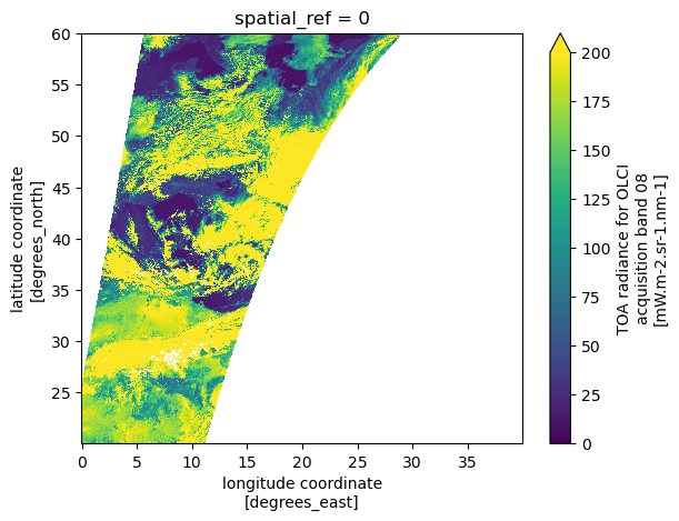
Open a Sentinel-3 SLSTR Level-2 LST
We now access a Sentinel-3 SLSTR Level-2 LST product in analysis mode. The data access methods shown above apply equally to Sentinel-3 SLSTR Level-2 LST.
Find a Sentinel-3 SLSTR Level-2 LST Zarr Sample via STAC
To obtain a product URL, you can use the STAC Browser to search for a Sentinel-3 SLSTR Level-2 LST tile.
catalog = pystac_client.Client.open("https://stac.core.eopf.eodc.eu")
items = list(
    catalog.search(
        collections=["sentinel-3-slstr-l2-lst"],
        bbox=[7.2, 44.5, 7.4, 44.7],
        datetime=[str(datetime.date.today() - datetime.timedelta(days=5)), None],
    ).items()
)
items
[<Item id=S3A_SL_2_LST____20260331T093213_20260331T093513_20260331T115031_0179_137_364_2160_PS1_O_NR_004>,
<Item id=S3A_SL_2_LST____20260330T212119_20260330T212419_20260331T000117_0179_137_357_0720_PS1_O_NR_004>,
<Item id=S3B_SL_2_LST____20260330T204237_20260330T204537_20260330T232628_0179_118_214_0720_ESA_O_NR_004>,
<Item id=S3A_SL_2_LST____20260330T095824_20260330T100124_20260330T122502_0179_137_350_2160_PS1_O_NR_004>,
<Item id=S3B_SL_2_LST____20260330T091943_20260330T092243_20260330T113544_0179_118_207_2160_ESA_O_NR_004>,
<Item id=S3A_SL_2_LST____20260329T214729_20260329T215029_20260330T003114_0179_137_343_0720_PS1_O_NR_004>,
<Item id=S3A_SL_2_LST____20260329T214729_20260329T215029_20260331T093531_0179_137_343_0720_PS1_O_NT_004>,
<Item id=S3B_SL_2_LST____20260329T210848_20260329T211148_20260329T235533_0179_118_200_0720_ESA_O_NR_004>,
<Item id=S3B_SL_2_LST____20260329T210848_20260329T211148_20260331T040837_0180_118_200_0720_ESA_O_NT_004>,
<Item id=S3A_SL_2_LST____20260329T102435_20260329T102735_20260329T125030_0179_137_336_2160_PS1_O_NR_004>,
<Item id=S3A_SL_2_LST____20260329T102435_20260329T102735_20260330T220124_0179_137_336_2160_PS1_O_NT_004>,
<Item id=S3B_SL_2_LST____20260329T094553_20260329T094853_20260329T121220_0179_118_193_2160_ESA_O_NR_004>,
<Item id=S3B_SL_2_LST____20260329T094553_20260329T094853_20260330T170121_0179_118_193_2160_ESA_O_NT_004>,
<Item id=S3B_SL_2_LST____20260328T213459_20260328T213759_20260329T001031_0179_118_186_0720_ESA_O_NR_004>,
<Item id=S3B_SL_2_LST____20260328T213459_20260328T213759_20260330T051647_0179_118_186_0720_ESA_O_NT_004>,
<Item id=S3A_SL_2_LST____20260328T203241_20260328T203541_20260328T231506_0179_137_328_0720_PS1_O_NR_004>,
<Item id=S3A_SL_2_LST____20260328T203241_20260328T203541_20260330T081257_0179_137_328_0720_PS1_O_NT_004>,
<Item id=S3B_SL_2_LST____20260328T101204_20260328T101504_20260328T123424_0179_118_179_2160_ESA_O_NR_004>,
<Item id=S3B_SL_2_LST____20260328T101204_20260328T101504_20260329T172450_0180_118_179_2160_ESA_O_NT_004>,
<Item id=S3A_SL_2_LST____20260327T205851_20260327T210151_20260329T083311_0179_137_314_0720_PS1_O_NT_004>,
<Item id=S3A_SL_2_LST____20260327T205851_20260327T210151_20260327T234107_0179_137_314_0720_PS1_O_NR_004>,
<Item id=S3A_SL_2_LST____20260327T093557_20260327T093857_20260328T204053_0179_137_307_2160_PS1_O_NT_004>,
<Item id=S3A_SL_2_LST____20260327T093557_20260327T093857_20260327T120121_0180_137_307_2160_PS1_O_NR_004>,
<Item id=S3A_SL_2_LST____20260326T212502_20260326T212802_20260328T091525_0179_137_300_0720_PS1_O_NT_004>,
<Item id=S3A_SL_2_LST____20260326T212502_20260326T212802_20260327T000636_0179_137_300_0720_PS1_O_NR_004>,
<Item id=S3B_SL_2_LST____20260326T204621_20260326T204921_20260328T030457_0179_118_157_0720_ESA_O_NT_004>,
<Item id=S3B_SL_2_LST____20260326T204621_20260326T204921_20260326T232930_0180_118_157_0720_ESA_O_NR_004>,
<Item id=S3A_SL_2_LST____20260326T100207_20260326T100507_20260327T212028_0180_137_293_2160_PS1_O_NT_004>,
<Item id=S3A_SL_2_LST____20260326T100207_20260326T100507_20260326T122451_0179_137_293_2160_PS1_O_NR_004>,
<Item id=S3B_SL_2_LST____20260326T092326_20260326T092626_20260327T153634_0179_118_150_2160_ESA_O_NT_004>,
<Item id=S3B_SL_2_LST____20260326T092326_20260326T092626_20260326T114832_0179_118_150_2160_ESA_O_NR_004>]item = items[0]Open Sentinel-3 SLSTR Level-2 LST with Default Parameters
We can now open the Sentinel-3 product in analysis mode using the xr.open_dataset method, as before.
ds = xr.open_dataset(
    item.assets["product"].href,
    engine="eopf-zarr",
    chunks={},
)
dsAs an example, we plot the LST array, which triggers data loading, rectification, and visualization of the rectified result.
ds.lst.plot()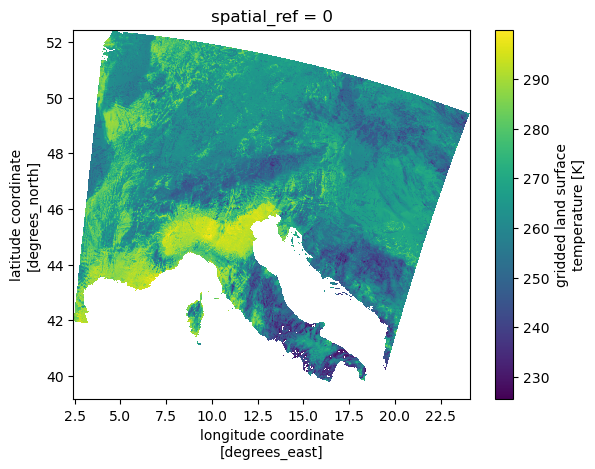
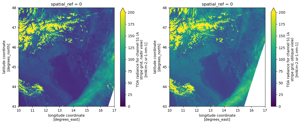
Open Sentinel-3 SLSTR Level-1B RBT
We now access a Sentinel-3 SLSTR Level-1B RBT product in analysis mode.
The SLSTR instrument provides observations from two viewing geometries: nadir and oblique (forward view). These are designed to improve atmospheric correction and enable more accurate surface measurements.
Accordingly, many variables in the RBT product are available in pairs:
*_an→ nadir view (e.g.s1_radiance_an)*_ao→ oblique view (e.g.s1_radiance_ao)
Find a Sentinel-3 SLSTR Level-1B RBT Zarr Sample via STAC
To obtain a product URL, you can use the STAC Browser to search for a Sentinel-3 SLSTR Level-1B RBT tile.
catalog = pystac_client.Client.open("https://stac.core.eopf.eodc.eu")
items = list(
    catalog.search(
        collections=["sentinel-3-slstr-l1-rbt"],
        bbox=[7.2, 44.5, 7.4, 44.7],
        datetime=[str(datetime.date.today() - datetime.timedelta(days=6)), None],
    ).items()
)
items
[<Item id=S3A_SL_1_RBT____20260331T093213_20260331T093513_20260331T114729_0179_137_364_2160_PS1_O_NR_004>,
<Item id=S3A_SL_1_RBT____20260330T212119_20260330T212419_20260330T235516_0179_137_357_0720_PS1_O_NR_004>,
<Item id=S3B_SL_1_RBT____20260330T204237_20260330T204537_20260330T230942_0179_118_214_0720_ESA_O_NR_004>,
<Item id=S3A_SL_1_RBT____20260330T095824_20260330T100124_20260330T121923_0179_137_350_2160_PS1_O_NR_004>,
<Item id=S3B_SL_1_RBT____20260330T091943_20260330T092243_20260330T113200_0179_118_207_2160_ESA_O_NR_004>,
<Item id=S3A_SL_1_RBT____20260329T214729_20260329T215029_20260330T002523_0179_137_343_0720_PS1_O_NR_004>,
<Item id=S3A_SL_1_RBT____20260329T214729_20260329T215029_20260331T091614_0179_137_343_0720_PS1_O_NT_004>,
<Item id=S3B_SL_1_RBT____20260329T210848_20260329T211148_20260329T235156_0179_118_200_0720_ESA_O_NR_004>,
<Item id=S3B_SL_1_RBT____20260329T210848_20260329T211148_20260331T020244_0180_118_200_0720_ESA_O_NT_004>,
<Item id=S3A_SL_1_RBT____20260329T102435_20260329T102735_20260329T124343_0179_137_336_2160_PS1_O_NR_004>,
<Item id=S3A_SL_1_RBT____20260329T102435_20260329T102735_20260330T214438_0179_137_336_2160_PS1_O_NT_004>,
<Item id=S3B_SL_1_RBT____20260329T094553_20260329T094853_20260330T144539_0179_118_193_2160_ESA_O_NT_004>,
<Item id=S3B_SL_1_RBT____20260329T094553_20260329T094853_20260329T120822_0179_118_193_2160_ESA_O_NR_004>,
<Item id=S3B_SL_1_RBT____20260328T213459_20260328T213759_20260329T000337_0179_118_186_0720_ESA_O_NR_004>,
<Item id=S3B_SL_1_RBT____20260328T213459_20260328T213759_20260330T031418_0179_118_186_0720_ESA_O_NT_004>,
<Item id=S3A_SL_1_RBT____20260328T203241_20260328T203541_20260328T230845_0179_137_328_0720_PS1_O_NR_004>,
<Item id=S3A_SL_1_RBT____20260328T203241_20260328T203541_20260330T075507_0179_137_328_0720_PS1_O_NT_004>,
<Item id=S3B_SL_1_RBT____20260328T101204_20260328T101504_20260328T122852_0179_118_179_2160_ESA_O_NR_004>,
<Item id=S3B_SL_1_RBT____20260328T101204_20260328T101504_20260329T152553_0180_118_179_2160_ESA_O_NT_004>,
<Item id=S3A_SL_1_RBT____20260327T205851_20260327T210151_20260329T081139_0179_137_314_0720_PS1_O_NT_004>,
<Item id=S3A_SL_1_RBT____20260327T205851_20260327T210151_20260327T233553_0179_137_314_0720_PS1_O_NR_004>,
<Item id=S3A_SL_1_RBT____20260327T093557_20260327T093857_20260328T202525_0179_137_307_2160_PS1_O_NT_004>,
<Item id=S3A_SL_1_RBT____20260327T093557_20260327T093857_20260327T115450_0180_137_307_2160_PS1_O_NR_004>,
<Item id=S3A_SL_1_RBT____20260326T212502_20260326T212802_20260328T085624_0179_137_300_0720_PS1_O_NT_004>,
<Item id=S3A_SL_1_RBT____20260326T212502_20260326T212802_20260327T000043_0179_137_300_0720_PS1_O_NR_004>,
<Item id=S3B_SL_1_RBT____20260326T204621_20260326T204921_20260328T011313_0179_118_157_0720_ESA_O_NT_004>,
<Item id=S3B_SL_1_RBT____20260326T204621_20260326T204921_20260326T231336_0180_118_157_0720_ESA_O_NR_004>,
<Item id=S3A_SL_1_RBT____20260326T100207_20260326T100507_20260327T210433_0180_137_293_2160_PS1_O_NT_004>,
<Item id=S3A_SL_1_RBT____20260326T100207_20260326T100507_20260326T121940_0179_137_293_2160_PS1_O_NR_004>,
<Item id=S3B_SL_1_RBT____20260326T092326_20260326T092626_20260327T133632_0179_118_150_2160_ESA_O_NT_004>,
<Item id=S3B_SL_1_RBT____20260326T092326_20260326T092626_20260326T114459_0179_118_150_2160_ESA_O_NR_004>,
<Item id=S3B_SL_1_RBT____20260325T211231_20260325T211531_20260327T011844_0179_118_143_0720_ESA_O_NT_004>,
<Item id=S3B_SL_1_RBT____20260325T211231_20260325T211531_20260325T234058_0179_118_143_0720_ESA_O_NR_004>,
<Item id=S3A_SL_1_RBT____20260325T102818_20260325T103118_20260326T215932_0180_137_279_2160_PS1_O_NT_004>,
<Item id=S3A_SL_1_RBT____20260325T102818_20260325T103118_20260325T124603_0180_137_279_2160_PS1_O_NR_004>,
<Item id=S3B_SL_1_RBT____20260325T094937_20260325T095237_20260326T143122_0179_118_136_2160_ESA_O_NT_004>,
<Item id=S3B_SL_1_RBT____20260325T094937_20260325T095237_20260325T121153_0179_118_136_2160_ESA_O_NR_004>]item = items[-1]Open Sentinel-3 SLSTR Level-1B RBT with Default Parameters
We can now open the Sentinel-3 product in analysis mode using the xr.open_dataset method, as before.
ds = xr.open_dataset(
    item.assets["product"].href,
    engine="eopf-zarr",
    chunks={},
    bbox=[10, 43, 17, 48],
)
dsAs an example, we plot the nadir and oblique views of the S1 thermal channel side by side.
%%time
fig, ax = plt.subplots(1, 2, figsize=(12, 5))
ds.s1_radiance_an.plot(ax=ax[0], vmin=0, vmax=200)
ds.s1_radiance_ao.plot(ax=ax[1], vmin=0, vmax=200)
plt.tight_layout()
CPU times: user 1.41 s, sys: 64.4 ms, total: 1.47 s
Wall time: 1.12 s
Other Sentinel-3 products can be accessed using the same approach and are therefore not shown here in detail.
Conclusion
This notebook demonstrates how to access Sentinel-2 EOPF Zarr samples in analysis mode using the xarray-eopf plugin. The key takeaways are:
Analysis mode is the default
op_mode.In analysis mode, Sentinel-3 spectral bands are rectified to a rectilinear grid
Data can be accessed lazily at a user-defined resolution, bounding box, and CRS, enabling flexible resampling, subsetting, and reprojection.
Note: This notebook only covers analysis mode for Sentinel-3. To learn more about native mode, see the Sentinel-3 native mode notebook.
