OSI - Oil Spill Index

Table of contents¶

Introduction
Setup
STAC search
Create Datacube
Spatial and temporal filtering
Cloud masking
Visualize masked data for one date
Compute OSI
Visualize results

Run this notebook interactively with all dependencies pre-installed

Introduction¶

The OSI (Oil Spill Index) uses visible Sentinel-2 bands to display oil spills over water in the costal/marine environment. The OSI is constructed by summing-up the bands representing the shoulders of absorption features of oil as numerator and the band located nearest to the absorption feature as denominator to discriminate oil spill as below.

OSI = (B03 + B04) / B02

The original idea was created by Sankaran Rajendran and is available in the Sentinel Hub documentation here.

MV Wakashio oil spill¶

Source: International Maritime Organization 2020 link

This notebook demonstrates the application of the Oil Spill Index (OSI) to the MV Wakashio oil spill incident in Mauritius using Sentinel-2 imagery.

The incident occured in July 2020 when a Japanese ship ran aground on a coral reef and started leaking fuel oil into the surrounding area for several days.

MV Wakashio was 300 meters long and at the time was carrying roughly 4000 tons of very low sulfur fuel oil (VLSFO). High winds and waves made the cleanup process very difficult.

More information on the oil spill can be found here:

United Nations Office for the Coordination of Humanitarian Affairs (OCHA) - Oil Spill in Mauritius

Setup¶

Start importing the necessary libraries

import xarray as xr
from datetime import datetime
import geopandas as gpd
import matplotlib.pyplot as plt
import numpy as np
import pystac_client
from pystac_client import CollectionSearch

from shapely import geometry

from distributed import LocalCluster

cluster = LocalCluster(processes=False)
client = cluster.get_client()
cluster

STAC search¶

search = CollectionSearch(
    url="https://stac.core.eopf.eodc.eu/collections",
)
for collection_dict in search.collections_as_dicts():
    print(collection_dict["id"])

sentinel-2-l2a
sentinel-3-slstr-l2-lst
sentinel-3-olci-l2-lfr
sentinel-2-l1c
sentinel-3-slstr-l1-rbt
sentinel-3-olci-l1-efr
sentinel-3-olci-l1-err
sentinel-1-l1-slc
sentinel-1-l1-grd
sentinel-1-l2-ocn
sentinel-3-olci-l2-lrr

catalog = pystac_client.Client.open("https://stac.core.eopf.eodc.eu")
items = list(
    catalog.search(
        collections=["sentinel-2-l2a"],
        bbox=[
            57.684646751857144,
            -20.466450832612153,
            57.78531132251502,
            -20.3794154117235,
        ],
        datetime=["2020-06-30", "2020-10-01"],
    ).items()
)
print(f"items found: {len(items)}")

dates = [
    datetime(2020, 7, 17),
    datetime(2020, 8, 1),
    datetime(2020, 8, 6),
    datetime(2020, 9, 5),
]

date_set = {d.date() for d in dates}

items = [i for i in items if i.datetime.date() in date_set]
print(f"Selected items: {len(items)}")

items found: 19
Selected items: 4

items

[<Item id=S02MSIL2A_20200905T062449_0000_B091_T778>,
 <Item id=S02MSIL2A_20200806T062449_0000_B091_T103>,
 <Item id=S02MSIL2A_20200801T062451_0000_A091_T114>,
 <Item id=S02MSIL2A_20200717T062449_0000_B091_T774>]

Create Datacube¶

In the following section we extract the 20 meter bands as well as the scene classification layer (scl) from the Sentinel-2 data.

These variables are then merged into a single datacube

datasets = []
for item in items:
    href = item.assets["product"].href

    ds = xr.open_datatree(href, engine="zarr", chunks={}, mask_and_scale=True)

    ds_ref = ds["measurements"]["reflectance"]["r20m"].ds

    ds_ref = ds_ref.assign_coords(time=item.datetime).expand_dims("time")
    datasets.append(ds_ref)

r20m = xr.concat(datasets, dim="time")

scl_datasets = []

for item in items:
    href = item.assets["product"].href

    ds = xr.open_datatree(href, engine="zarr", chunks={}, mask_and_scale=True)

    ds_scl = ds["conditions"]["mask"]["l2a_classification"]["r20m"].ds

    ds_scl = ds_scl.assign_coords(time=item.datetime).expand_dims("time")
    scl_datasets.append(ds_scl)


scl_cube = xr.concat(scl_datasets, dim="time")

datacube = xr.merge([r20m, scl_cube])
datacube = datacube.sortby("time")

datacube

Spatial and temporal filtering¶

epsg_code = items[0].properties.get("proj:code")


def spatial_filter(ds: xr.DataArray, bbox: list, epsg: int = 32740):
    x_slice = slice(bbox[0], bbox[2])
    y_slice = slice(bbox[3], bbox[1])
    bbox_polygon = geometry.box(*bbox)
    polygon = gpd.GeoDataFrame(index=[0], crs="epsg:4326", geometry=[bbox_polygon])
    bbox_reproj = polygon.to_crs("epsg:" + str(epsg)).geometry.values[0].bounds
    x_slice = slice(bbox_reproj[0], bbox_reproj[2])
    y_slice = slice(bbox_reproj[3], bbox_reproj[1])
    return ds.sel(x=x_slice, y=y_slice)


def temporal_filter(ds: xr.DataArray, date):
    return ds.sel(time=date, method="nearest")


dates = ["2020-07-17", "2020-08-01", "2020-08-06", "2020-09-05"]

bbox = [57.684646751857144, -20.466450832612153, 57.78531132251502, -20.3794154117235]

datasets = []

for date in dates:
    ds_spatial = spatial_filter(datacube, bbox)
    ds_temporal = temporal_filter(ds_spatial, date)
    datasets.append(ds_temporal)

datasets[0]

Cloud masking¶

masked_datasets = []

for ds in datasets:

    scl = ds["scl"]

    cloud_mask = ~scl.isin([3, 8, 9, 10])

    bands = [v for v in ds.data_vars if v != "scl"]
    ds_masked = ds[bands].where(cloud_mask)

    masked_datasets.append(ds_masked)

masked_datasets[0]

Visualize masked data for one date¶

The following visualization shows the area of interest before the oilspill event.

def compute_rgb(dataset):
    b02 = dataset["b02"]
    b03 = dataset["b03"]
    b04 = dataset["b04"]

    rgb = np.stack([b04, b03, b02], axis=-1)

    rgb = (rgb / 0.25).clip(0, 1)

    plt.figure(figsize=(10, 10))
    plt.imshow(rgb, origin="upper")
    plt.title("RGB composite before the oil spill")
    plt.axis("off")
    plt.show()


ds = masked_datasets[0]
compute_rgb(ds)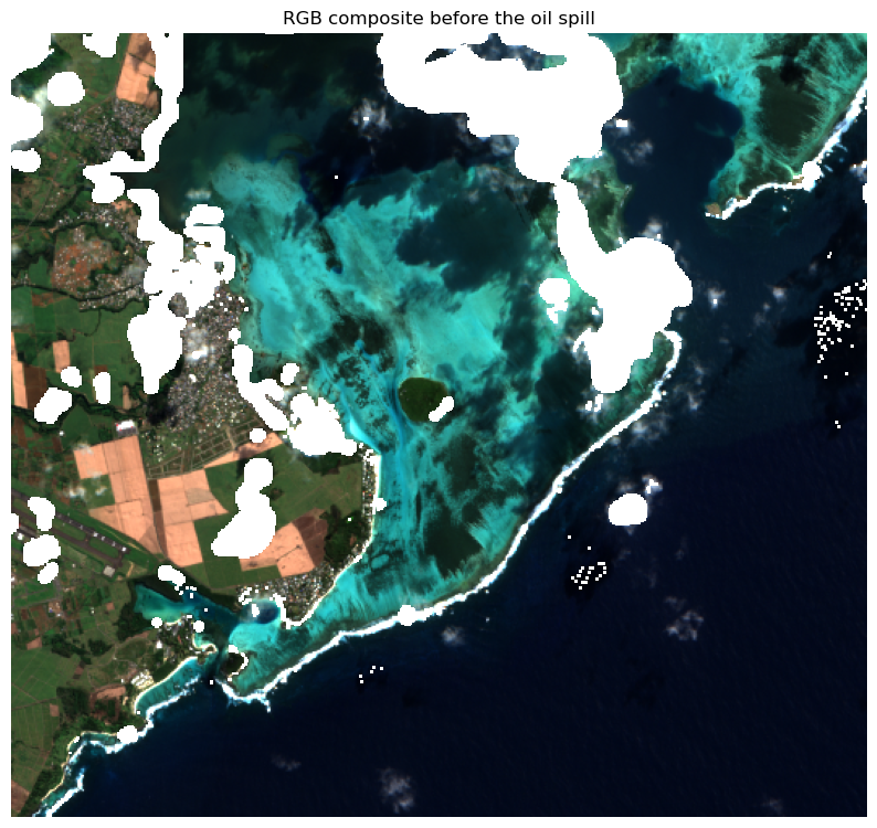

Compute OSI¶

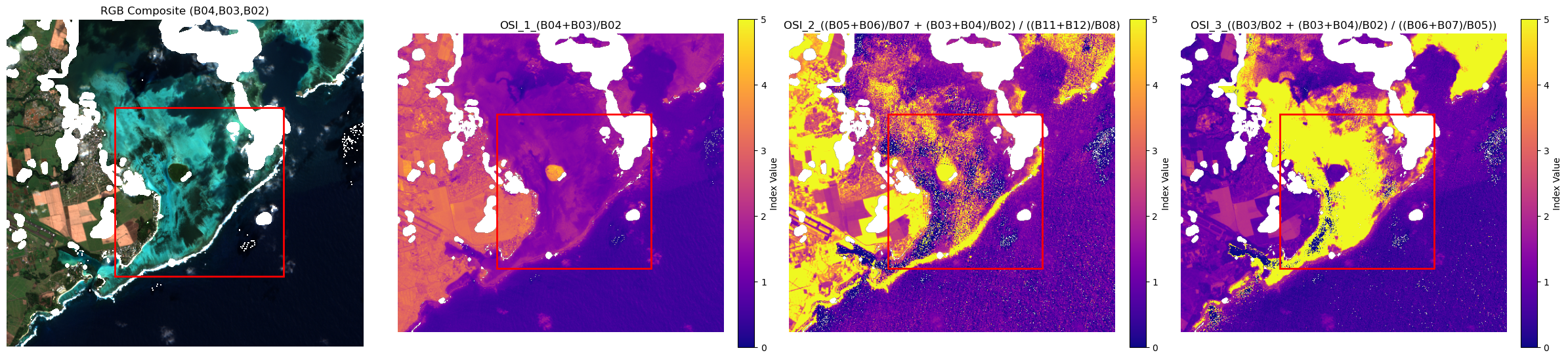
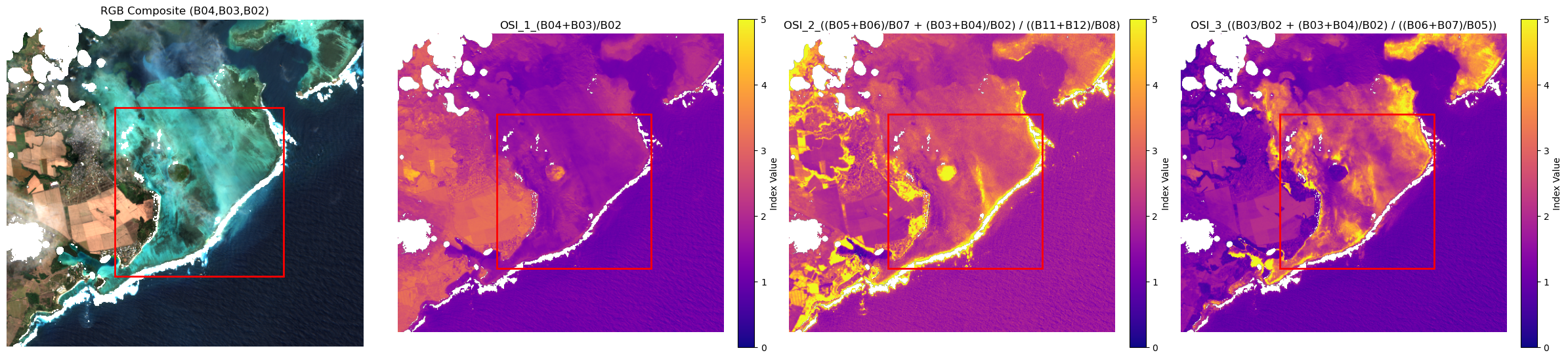
The standard way of computing OSI is (B03 + B04) / B02.

However, there are several other variants that can be used to compute the OSI, taking advantage of different spectral bands. These variants may provide additional insights or improve the sensitivity of the index to oil spills:

R: (B05+ B06)/ B07; G: (B03+ B04)/B02; B: (B011+ B012)/ B08

R: B03/ B02; G: (B03+ B04)/B02; B: (B06+ B07)/ B05

Zakzouk, M., Abou El-Magd, I., Ali, E. M., Abdulaziz, A. M., Rehman, A., & Saba, T. (2024). Novel oil spill indices for sentinel-2 imagery: A case study of natural seepage in Qaruh Island, Kuwait. MethodsX, 12, 102520.

In this example we compute all variants and visualize them below

import matplotlib.patches as patches


def compute_osi_variants(dataset, highlight_box=None):
    b02 = dataset["b02"]
    b03 = dataset["b03"]
    b04 = dataset["b04"]
    b05 = dataset["b05"]
    b06 = dataset["b06"]
    b07 = dataset["b07"]
    b08 = dataset["b8a"]
    b11 = dataset["b11"]
    b12 = dataset["b12"]

    osi_variants = {}

    # Variant 1: (B04 + B03) / B02
    osi_variants["OSI_1_(B04+B03)/B02"] = (b04 + b03) / b02

    # Variant 2
    R = (b05 + b06) / b07
    G = (b03 + b04) / b02
    B = (b11 + b12) / b08
    osi_variants["OSI_2_((B05+B06)/B07 + (B03+B04)/B02) / ((B11+B12)/B08)"] = (
        R + G
    ) / B

    # Variant 3
    R = b03 / b02
    G = (b03 + b04) / b02
    B = (b06 + b07) / b05
    osi_variants["OSI_3_((B03/B02 + (B03+B04)/B02) / ((B06+B07)/B05))"] = (R + G) / B

    rgb = np.stack([b04, b03, b02], axis=-1).astype(float)
    rgb = (rgb / 0.25).clip(0, 1)  # simple linear stretch

    # Combine RGB + OSI variants for plotting
    n = len(osi_variants) + 1
    fig, axes = plt.subplots(1, n, figsize=(6 * n, 6))
    if n == 1:
        axes = [axes]

    # Add red box
    def add_highlight(ax):
        if highlight_box:
            x, y, w, h = highlight_box
            rect = patches.Rectangle(
                (x, y), w, h, linewidth=2, edgecolor="red", facecolor="none"
            )
            ax.add_patch(rect)

    # Plot RGB
    axes[0].imshow(rgb, origin="upper")
    axes[0].set_title("RGB Composite (B04,B03,B02)")
    axes[0].axis("off")
    add_highlight(axes[0])

    # Plot OSI variants
    for ax, (name, osi) in zip(axes[1:], osi_variants.items()):
        im = ax.imshow(osi, cmap="plasma", vmin=0, vmax=5)
        ax.set_title(name)
        ax.axis("off")
        fig.colorbar(im, ax=ax, fraction=0.046, pad=0.04, label="Index Value")
        add_highlight(ax)

    plt.tight_layout()
    plt.show()

    return osi_variants

Visualize results¶

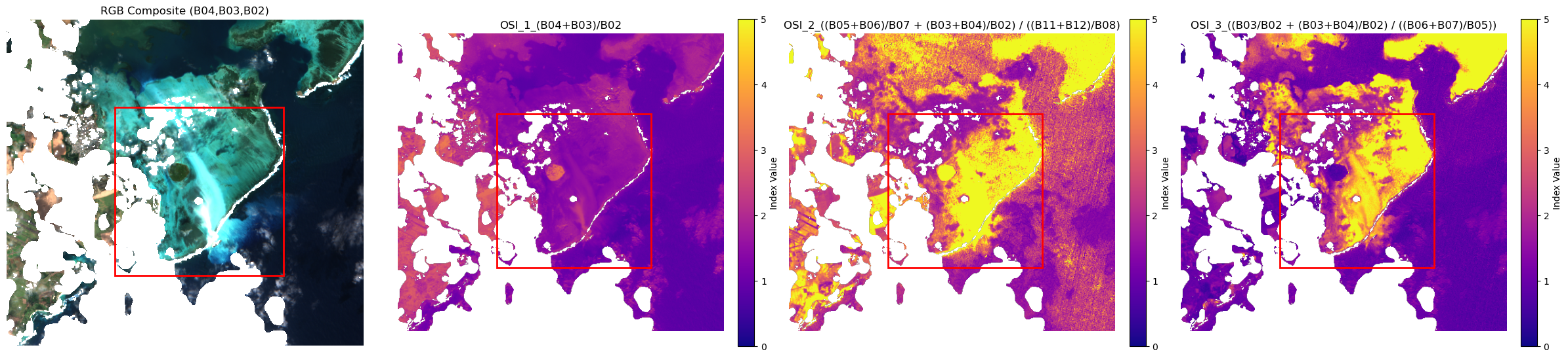
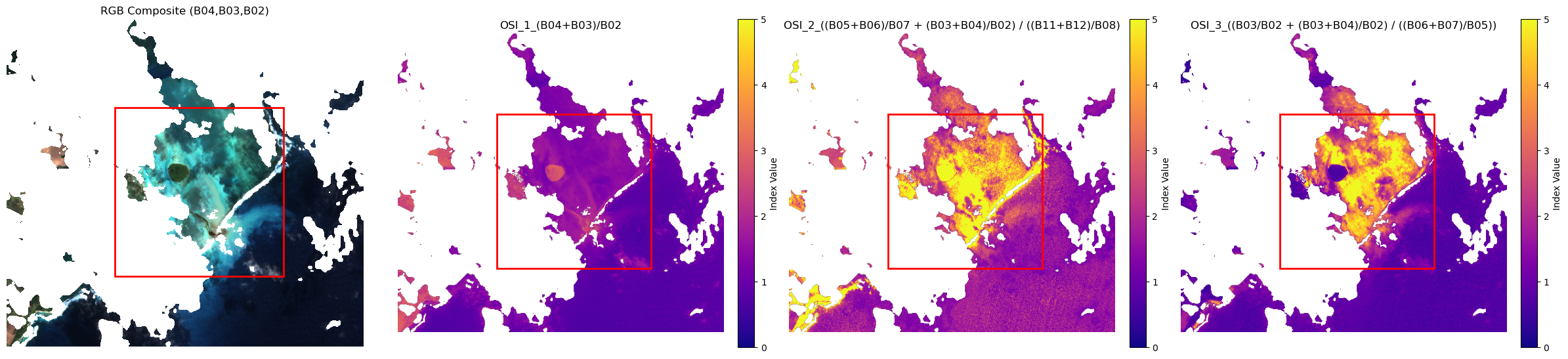
In the following visualizations we can see the different OSI variants computed from the Sentinel-2 imagery for each of the 4 dates.

The more classical approach does show some distinction between oil spill and non-oil spill areas.

Variant two shows a more pronounced separation between the two classes, indicating its potential effectiveness in detecting oil spills, however, it also highlights the land which may not be ideal.

Variant three appears to visibly show oil spill and non oilspill areas while leaving the land areas less pronounced.

for i in range(4):
    ds = masked_datasets[i]
    print(f"Displayed OSI variants for date: {ds.time.values}")
    compute_osi_variants(ds, highlight_box=(160, 130, 250, 250))

Displayed OSI variants for date: 2020-07-17T06:24:49.024000000

Displayed OSI variants for date: 2020-08-01T06:24:51.024000000

Displayed OSI variants for date: 2020-08-06T06:24:49.024000000

Displayed OSI variants for date: 2020-09-05T06:24:49.024000000

# close the dask cluster
cluster.close()

Welcome

Transforming workflow for oceanography study using Sentinel‑2 data, from SAFE to Zarr

Welcome

NDVI Time-Series Analysis of Potato Fields