NDVI Time-Series Analysis of Potato Fields
A step-by-step guide to extracting and analyzing temporal NDVI profiles from potato fields for crop-type studies.

Table of contents
Run this notebook interactively with all dependencies pre-installed
Preface
The original notebook used as a starting point for this work is a openEO platform example, available here. The example has been adapted to use the data provided by the EOPF Zarr Samples project instead of the openEO API.
Introduction
This notebook demonstrates how to perform NDVI time-series analysis for potato fields using EOPF-ZARR Sentinel-2 Level-2A data. The focus is on extracting clean vegetation profiles that highlight the characteristic temporal patterns of potato growth. These profiles can later serve as input features for crop-type classification.
The workflow is structured as follows:
Data access: Connect to a STAC catalog and query Sentinel-2 scenes for a specific field and time range.
Preprocessing: Use the Scene Classification Layer (SCL) with an openEO-style
mask_scl_dilationto remove clouds, shadows, snow, and other unwanted contamination.NDVI computation: Derive NDVI from red (B04) and near-infrared (B08) bands, optionally scaling to match openEO conventions.
Temporal aggregation: Aggregate NDVI values into dekads (10-day periods), interpolate missing data, and filter to a specific season.
Analysis & visualization: Plot the field-mean NDVI profile with uncertainty, revealing the phenological stages of potato development.
This pipeline demonstrates how to transform raw Earth Observation data into interpretable temporal signals, laying the groundwork for future rule-based or machine learning-based crop classification.
Timeseries analysis of vegetation greenness
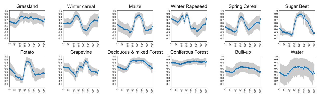
Different land cover types can be identified by their seasonal green-up and green-down patterns. NDVI time series capture these phenological dynamics:
Coniferous forests remain green all year round, showing little variation in NDVI.
Grasslands show moderate seasonal cycles with higher values in spring and summer.
Annual crops (e.g., sugar beet, maize, potato) exhibit strong seasonal fluctuations, with steep green-up during growth, a pronounced peak, and rapid decline after harvest.
An overview of NDVI trajectories for several crop types is shown in the plots below. These illustrate how temporal profiles can serve as fingerprints for distinguishing between vegetation classes.
Setup
Start importing the necessary libraries
import os
import xarray as xr
from datetime import datetime
import matplotlib.pyplot as plt
import numpy as np
import pandas as pd
import pystac_client
from scipy import ndimage as ndi
from distributed import LocalCluster
from pyproj import Transformer
cluster = LocalCluster(processes=False)
client = cluster.get_client()
cluster/home/mclaus@eurac.edu/micromamba/envs/eopf-zarr/lib/python3.11/site-packages/distributed/node.py:187: UserWarning: Port 8787 is already in use.
Perhaps you already have a cluster running?
Hosting the HTTP server on port 36871 instead
warnings.warn(
Area of Interest
The region of interest is located over the Belgium 31N tile, referenced in EPSG:32631. For the STAC query, the required input is the bounding box in EPSG:4326 (bbox_4326). Meanwhile, UTM-based slices are generated to subset the dataset, which is natively stored in UTM coordinates.
# Define AOI and convert to raster CRS
spatial_extent = {
    "west": 3.547150,
    "south": 50.865238,
    "east": 3.548602,
    "north": 50.866717,
}

bbox_4326 = [
    spatial_extent["west"],
    spatial_extent["south"],
    spatial_extent["east"],
    spatial_extent["north"],
]

# Convert AOI to UTM 33N (same as Sentinel-2 data)
transformer = Transformer.from_crs("EPSG:4326", "EPSG:32631", always_xy=True)
west_utm, south_utm = transformer.transform(
    spatial_extent["west"], spatial_extent["south"]
)
east_utm, north_utm = transformer.transform(
    spatial_extent["east"], spatial_extent["north"]
)

# Spatial slice parameters
x_slice = slice(west_utm, east_utm)
y_slice = slice(north_utm, south_utm)
STAC Search
# Connect to the STAC catalog
catalog = pystac_client.Client.open("https://stac.core.eopf.eodc.eu")

# Search for Sentinel-2 L2A items within a specific bounding box and date range
search = catalog.search(
    collections=["sentinel-2-l2a"],
    bbox=bbox_4326,
    datetime="2018-11-01/2020-02-01",
)

# Retrieve the list of matching items
items = list(search.items())
hrefs = [item.assets["product"].href for item in items]
print(f"List of first Five Items returned from the STAC query: {items[:5]}")
print(f"List of first Five Zarr URLs returned from the STAC query: {hrefs[:5]}")List of first Five Items returned from the STAC query: [<Item id=S02MSIL2A_20200131T105251_0000_A051_T973>, <Item id=S02MSIL2A_20200129T110209_0000_B094_T881>, <Item id=S02MSIL2A_20200126T105229_0000_B051_T215>, <Item id=S02MSIL2A_20200124T110331_0000_A094_T671>, <Item id=S02MSIL2A_20200121T105341_0000_A051_T512>]
List of first Five Zarr URLs returned from the STAC query: ['https://objects.eodc.eu/e05ab01a9d56408d82ac32d69a5aae2a:notebook-data/tutorial_data/cpm_v260/S2A_MSIL2A_20200131T105251_N0500_R051_T31UES_20230426T102522.zarr', 'https://objects.eodc.eu:443/e05ab01a9d56408d82ac32d69a5aae2a:notebook-data/tutorial_data/cpm_v260/S2B_MSIL2A_20200129T110209_N0500_R094_T31UES_20230628T193235.zarr', 'https://objects.eodc.eu:443/e05ab01a9d56408d82ac32d69a5aae2a:notebook-data/tutorial_data/cpm_v260/S2B_MSIL2A_20200126T105229_N0500_R051_T31UES_20230428T121217.zarr', 'https://objects.eodc.eu:443/e05ab01a9d56408d82ac32d69a5aae2a:notebook-data/tutorial_data/cpm_v260/S2A_MSIL2A_20200124T110331_N0500_R094_T31UES_20230428T065124.zarr', 'https://objects.eodc.eu:443/e05ab01a9d56408d82ac32d69a5aae2a:notebook-data/tutorial_data/cpm_v260/S2A_MSIL2A_20200121T105341_N0500_R051_T31UES_20230427T135726.zarr']
DataCube Creation
def extract_time(ds):
    date_format = "%Y%m%dT%H%M%S"
    filename = ds.encoding["source"]
    date_str = os.path.basename(filename).split("_")[2]
    time = datetime.strptime(date_str, date_format)
    return ds.assign_coords(time=time)


datacube = xr.open_mfdataset(
    hrefs,
    engine="zarr",
    chunks={},
    group="/measurements/reflectance/r10m",
    concat_dim="time",
    combine="nested",
    preprocess=extract_time,
    mask_and_scale=True,
).sortby("time", ascending=True)

datacube = datacube[["b04", "b08"]].sel(x=x_slice, y=y_slice)
datacubescl = xr.open_mfdataset(
hrefs,
engine="zarr",
chunks={},
group="/conditions/mask/l2a_classification/r20m", # Adjust if necessary
concat_dim="time",
combine="nested",
preprocess=extract_time,
mask_and_scale=True,
).sortby("time", ascending=True)[["scl"]]
scl_resampled = scl.scl.interp_like(datacube, method="nearest")
datacube["scl"] = scl_resampled
datacube = datacube.compute()
datacube/home/mclaus@eurac.edu/micromamba/envs/eopf-zarr/lib/python3.11/site-packages/distributed/client.py:3371: UserWarning: Sending large graph of size 56.08 MiB.
This may cause some slowdown.
Consider loading the data with Dask directly
or using futures or delayed objects to embed the data into the graph without repetition.
See also https://docs.dask.org/en/stable/best-practices.html#load-data-with-dask for more information.
warnings.warn(
Applying Custom Mask SCL Dilation Process
def circular_kernel(radius: int) -> np.ndarray:
    """Create a 2D circular (disk) kernel with given radius in pixels."""
    r = int(radius)
    y, x = np.ogrid[-r : r + 1, -r : r + 1]
    k = (x * x + y * y) <= (r * r)
    return k.astype(np.float32)


def _dilate_with_convolve(mask_2d: np.ndarray, kernel: np.ndarray) -> np.ndarray:
    """
    Dilate a boolean mask using convolution with a (0/1) kernel.
    Returns a boolean array where any overlap with the kernel sets True.
    """
    if mask_2d.dtype != np.float32:
        mask_2d = mask_2d.astype(np.float32, copy=False)
    # Convolution counts how many True pixels fall under the kernel footprint.
    conv = ndi.convolve(mask_2d, kernel, mode="constant", cval=0.0)
    return conv > 0.0


def _apply_dilation_block(
    scl_block: np.ndarray, k1: np.ndarray, k2: np.ndarray
) -> np.ndarray:
    """
    Core block function (works on 2D arrays). Returns combined dilated mask (bool).
    Implements the openEO SCL logic used by mask_scl_dilation.
    """
    # S2 Sen2Cor SCL classes (for reference):
    #  0 NODATA, 1 SAT/DEF, 2 DARK, 3 CLOUD_SHADOW, 4 VEG, 5 NOT_VEG,
    #  6 WATER, 7 UNCLASS, 8 CLOUD_MED, 9 CLOUD_HIGH, 10 THIN_CIRRUS, 11 SNOW
    # openEO mask_scl_dilation uses:
    #   mask1 = everything except {2,4,5,6,7}  (aggressive neighbourhood removal)
    #   mask2 = {3,8,9,10,11}                  (clouds, shadows, snow)
    scl = scl_block.astype(np.int16, copy=False)

    mask1 = (scl != 2) & (scl != 4) & (scl != 5) & (scl != 6) & (scl != 7)
    mask2 = (scl == 3) | (scl == 8) | (scl == 9) | (scl == 10) | (scl == 11)

    dil1 = _dilate_with_convolve(mask1, k1)
    dil2 = _dilate_with_convolve(mask2, k2)

    combined = dil1 | dil2
    return combined


def mask_scl_dilation(
    ds: xr.Dataset, *, time_band_name: str = "time", scl_band_name: str = "scl"
) -> xr.Dataset:
    """
    Apply the mask_scl_dilation to an xarray Dataset containing a Sentinel-2 SCL band.

    Parameters
    ----------
    ds : xr.Dataset
        Must contain an integer SCL classification band.
        Expected dims include (y, x) and optionally time-like dims (e.g. t).
    time_band_name: str
        Name of the time dimension in 'ds'
    scl_band_name : str
        Name of the SCL band in `ds`.

    Returns
    -------
    xr.Dataset
        Same as input, with selected bands masked (set to NaN) wherever the dilated mask is True.
    """

    if scl_band_name not in ds:
        raise ValueError(
            f"{scl_band_name!r} not found in dataset variables: {list(ds.data_vars)}"
        )

    # Validate time dimension exists in dataset
    if time_band_name not in ds.dims:
        raise ValueError(
            f"{time_band_name!r} not found in dataset dimensions: {list(ds.dims)}"
        )

    kernel1 = circular_kernel(radius=8)
    kernel2 = circular_kernel(radius=100)

    scl = ds[scl_band_name]

    # Figure out which dims are spatial:
    # Try common names first, fallback to guessing the last two dims are (y, x)
    cand_xy = [d for d in ["y", "x"] if d in scl.dims]
    if len(cand_xy) != 2:
        # Guess last two dims in order
        cand_xy = list(scl.dims[-2:])
    ydim, xdim = cand_xy

    # Build dilated mask with apply_ufunc so it's Dask-friendly and vectorized over non-spatial dims.
    dilated = xr.apply_ufunc(
        _apply_dilation_block,
        scl,
        input_core_dims=[[ydim, xdim]],
        output_core_dims=[[ydim, xdim]],
        kwargs={"k1": kernel1.astype(np.float32), "k2": kernel2.astype(np.float32)},
        dask="parallelized",
        vectorize=True,
        output_dtypes=[bool],
        dask_gufunc_kwargs={"allow_rechunk": True},
    ).rename("dilated_mask")

    bands_to_mask = [v for v in ds.data_vars if v != scl_band_name]

    # Align masking array to each band (xarray broadcasting handles extra dims)
    out = ds.copy()
    for var in bands_to_mask:
        da = out[var]
        # Mask (set to NaN where dilated mask is True)
        # Preserve dtype for integer bands by promoting to float to allow NaNs
        if np.issubdtype(da.dtype, np.integer):
            da = da.astype(np.float32)
        out[var] = da.where(~dilated)

    out = out.drop_vars(scl_band_name)

    # Build a keep mask over time dimension
    keep = xr.concat(
        [out[v].notnull().any((ydim, xdim)) for v in bands_to_mask], dim="vars"
    ).any("vars")

    # Apply time filtering
    out = out.sel({time_band_name: keep})

    return out


# Usage examples
masked_ds = mask_scl_dilation(datacube, time_band_name="time", scl_band_name="scl")
masked_dsCompute NDVI
def compute_ndvi(ds: xr.Dataset) -> xr.DataArray:
    nir = ds["b08"].astype("float32")
    red = ds["b04"].astype("float32")
    num = nir - red
    den = nir + red
    ndvi = xr.where(den != 0, num / den, np.nan)
    ndvi.name = "NDVI"

    return ndvi


ndvi_dataset = compute_ndvi(masked_ds)
ndvi_datasetTemporal Aggregation of NDVI
def aggregate_to_dekad(ds: xr.Dataset, time_dim="time") -> xr.Dataset:
    """
    Group by dekad (10-day periods) and compute mean NDVI.
    """
    # Create dekad labels
    time_index = ds[time_dim].to_index()
    dekad_labels = [f"{d.year}-D{(d.dayofyear - 1) // 10 + 1:02}" for d in time_index]
    ds = ds.assign_coords(dekad=("time", dekad_labels))

    # Group by dekad and reduce
    agg_dekad = ds.groupby("dekad").mean(dim="time", keep_attrs=True)

    # Convert dekad labels back to timestamps (approximate mid-dekad date)
    dekad_dates = [
        pd.to_datetime(label.split("-D")[0])
        + pd.to_timedelta((int(label.split("-D")[1]) - 1) * 10 + 5, unit="D")
        for label in agg_dekad.dekad.values
    ]

    # Assign new 'time' coordinate and set it as index
    agg_dekad = (
        agg_dekad.assign_coords(time=("dekad", dekad_dates))
        .swap_dims({"dekad": "time"})
        .drop_vars("dekad")
    )

    return agg_dekad


agg_dekad = aggregate_to_dekad(ndvi_dataset)
agg_dekadTemporal Gap-Filling of Aggregated Mean NDVI
def interpolate_and_filter(ds: xr.Dataset, year: int, time_dim="time") -> xr.Dataset:
    """
    Linearly interpolate over missing dekads and filter to one calendar year.
    """
    # Ensure time is one chunk
    ds = ds.chunk({time_dim: -1})

    # Interpolate over time
    interpolated = ds.interpolate_na(
        dim=time_dim, method="linear", fill_value="extrapolate"
    )

    # Filter to calendar year
    start = f"{year}-01-01"
    end = f"{year}-12-31"
    return interpolated.sel({time_dim: slice(start, end)})


ndvi_dekad = interpolate_and_filter(agg_dekad, year=2019)
ndvi_dekadReducing Spatial Dimension
mean_df = ndvi_dekad.mean(dim=["x", "y"]).to_series()
std_df = ndvi_dekad.std(dim=["x", "y"]).to_series()
Visualising the Pattern
timeser = pd.concat([mean_df, std_df], axis=1).dropna()
timeser.columns = ["Mean NDVI", "SD"]
timeser.index = pd.to_datetime(timeser.index)
timeser = timeser.sort_index()

plt.plot(timeser["Mean NDVI"], "o-")
plt.fill_between(
    timeser.index,
    timeser["Mean NDVI"] - timeser["SD"],
    timeser["Mean NDVI"] + timeser["SD"],
    color="gray",
    alpha=0.2,
)
plt.ylim(0, 1)
plt.xticks(rotation=45)
plt.title("Potato")
plt.show()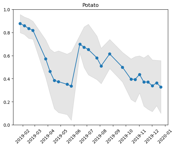
cluster.close()