Random Forest Based Land-Cover Mapping with Sentinel-2

Table of Contents¶

1. Introduction
2. Training Dataset Generation
3. Sample points selection
4. Read the points in Python
5. Satellite data retrieval
6. Predictors/Features extraction
7. Random Forest
8. Model training
9. Model prediction
10. Prediction Evaluation
11. What’s next?

Introduction¶

In this notebook, we will explore land cover mapping, a practice that has been integral to remote sensing since its inception. Land cover products are essential for studying the functional and morphological changes in Earth’s ecosystems and the environment, playing a crucial role in understanding climate change and carbon circulation (Congalton et al., 2014; Feddema et al., 2005; Sellers et al., 1997). Additionally, land cover mapping provides valuable information for policy development and a wide range of applications within the natural and life sciences, making it one of the most extensively studied applications in remote sensing (Yu et al., 2014; Tucker et al., 1985; Running, 2008; Yang et al., 2013). The diverse applications of land cover mapping lead to varied user needs. Depending on the specific use case, there can be significant differences in the desired target labels, the requested target year(s), the required output resolution, the feature set used, the stratification strategy employed, and more.

This exercise demonstrates how to efficiently use the Sentinel-2 EOPF Zarr products to implement a basic land cover classification.

Install the missing libraries

Training Dataset Generation¶

In this exercise, we will focus on 4 main classes:

1. artificial surfaces
2. agricultural areas
3. forests and seminatual areas
4. water bodies

The names of these classes comes from Corine Land Cover Level 0 classification scheme: https://wiki.openstreetmap.org/wiki/Corine_Land_Cover

Sample points selection¶

Generate 4 geoJSON files containing at least 10 points for each class using the website: https://geojson.io/#map=12/46.48882/11.33004

Follow this procedure for each land cover class:

1. Open the link: https://geojson.io/#map=12/46.48882/11.33004
2. Switch to satellite view selecting “Standard Satellite” as a base layer in the bottom left corner
3. Select the Draw Point tool and place a point in an area corresponding to the class
4. Repeat until you have at least 10 points
5. Save the geoJSON file with the top-left toolbar
6. Repeat for the other classes

Once that you have your 4 .geojson files, upload them to JupyterLab via drag & drop.

If you don’t want to do this small mapping exercise and skip directly to the next part, we prepared already the necessary files for the area of Bolzano, Italy.

Read the points in Python¶

Modify the file paths to match the files that you generated

Use GeoPandas to read the vector data. We also assign the corresponding Corine Land Cover code.

Inspect a GeoDataFrame object containing the sample points

Visualize a set of points to check if they are placed correctly on the corresponding class:

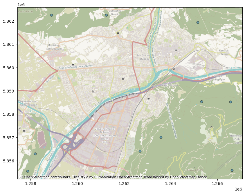
Satellite data retrieval¶

We will use optical Sentinel-2 data from the months of June, July and August 2022.

The data is available via the public EOPF Zarr STAC Catalog, available at https://stac.core.eopf.eodc.eu .

The xcube-eopf package will handle the STAC API requests and the datacube building parts.

We would like to extract the bounds of the area containing our training points.

To do that we can combine the different GeoDataFrames into a single one and use the total_bounds method.

Perform a temporal aggregation to get a monthly median of the data.

The median is capable to filter out data extremes, like clouds.
However, to get the best result is advisable to create and apply a cloud mask using the Scene Classification Layer, can you add this step before computing the median?

You can have a look at the example provided here: https://eopf-sample-service.github.io/eopf-sample-notebooks/sentinel-2-ndsi-snow-mapping/#cloud-snow

Remember to add the “scl” band when creating the datacube and to remove it before performing the feature extraction.

The default area above Bolzano corresponds to a manageable datacube which can fit easily in memory and therefore we will now load it in memory to speed up the next steps.

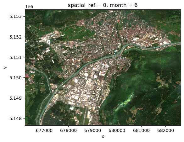
Visualize a sample image of the selected ones:

Predictors/Features extraction¶

Given the selected sample points and the Sentinel-2 data, we can now extract the data values corresponding to each sample point.

Each data array extracted will become a so-called predictor or feature vector.

Points - Data projection alignment¶

The geoJSON files contain points with coordinates expressed in lat/lon (WGS84 / EPSG:4326 coordinate system).

However, the data doesn’t necessarily has the same projection. Therefore, we reproject points to match data projection.

Feature Vector extraction¶

Given the reprojected points we can get the corresponding values and create feature vectors, which will be used for training.

We store the feature vectores in the same GeoDataFrame as the sampled points:

We perform some operations to:

1. Get the feature vector in the desired shape: NxM with N as the number of points and M the number of features (in this case bands*time)
2. Get the corresponding label vector with the correct format. The ML library we are using is expecting labels with values starting from 0 and therefore we have to map them.

Random Forest¶

We use the xgboost ML library with its Random Forest implementation.

For more info please read the documentation here:

https://xgboost.readthedocs.io/en/stable/tutorials/rf.html#standalone-random-forest-with-scikit-learn-like-api

and for the colsample_by* hyperparameters explanation check this nice article here:

https://medium.com/analytics-vidhya/xgboost-colsample-by-hyperparameters-explained-6c0bac1bdc1

Model training¶

Model prediction¶

To speed up the prediction process, we parallelize using xarray apply_ufunc, which allows to apply the same function call to multiple data chunks in parallel using Dask.

Prediction Evaluation¶

Now that our model has been trained and the prediction generated based on it, we can evaluate the result.

We didn’t do any split of the training set due to the limited number of samples, so we don’t have any test or validation set to use.

For this simple example, please evaluate the result using QGIS (or equivalent GIS software) and a satellite layer as a reference.

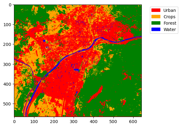
What’s next?¶

Now that you learned the basics, you can try to:

• Create and apply a cloud mask to the data in the Satellite data retrieval section.
• Apply the model to a new, unseen location and evaluate the results.
• Apply the model to a different year compared to the training set.