Transforming workflow for oceanography study using Sentinel‑2 data, from SAFE to Zarr

Table of contents¶

Introduction
Setup
Accessing Sentinel-2 Data in EOPF Zarr Format
Selecting a Region and Verifying Detector Consistency
Image Normalization and Whitecap Filtering
Fourier Transform & Welch-Based Spectral Analysis
🌊 Fourier and Cross-Spectral Analysis with angular metrics
Summary

Run this notebook interactively with all dependencies pre-installed

Introduction¶

This notebook demonstrates an improved workflow for oceanographic wave spectral analysis using Sentinel-2 data. We transition from the traditional SAFE format to the cloud-optimized EOPF Zarr format, highlighting substantial improvements in computational efficiency, simplicity, and scalability.

Original research workflow based on SAFE format is available at this notebook.

To understand the scientific background for the wave analysis methods used here, refer to: Kudryavtsev et al., 2016.

This workflow leverages the new EOPF Zarr format, eliminating the cumbersome steps required for loading SAFE files, significantly simplifying data handling and computational processing.

Setup and Dependencies¶

This notebook requires several Python libraries for data access, analysis, and visualization:

xarray, hvplot, holoviews for data access and visualization
pystac-client to query the STAC API
dask.distributed for scalable computation
numpy, matplotlib, skimage for numerics and filtering

In the EOPF JupyterHub environment, these packages are preinstalled. For local development, you may need to install them.

In the next cell, we start by importing the core Python libraries required for wave analysis, visualization, and efficient handling of large xarray datasets.

import xarray as xr
import hvplot.xarray
import pystac_client
import holoviews as hv
import numpy as np
import matplotlib.pyplot as plt
import cmocean
from skimage.filters import sobel
import matplotlib.colors as mcolors

hvplot.extension("bokeh")
# hvplot.extension("matplotlib")  # Uncomment for local development
# %matplotlib inline               # Uncomment for Matplotlib backend

# Uncomment the following lines to explicitly start a Dask LocalCluster
# and observe live behavior in the Dask JupyterLab extension.
# from dask.distributed import Client, LocalCluster\n",
# cluster = LocalCluster()   # Start a local Dask cluster
# client = Client(cluster)   # Connect to the cluster

# If you use JupyterHub, the link to your Dask dashboard looks like:
# /user/your_username/proxy/8787/

Loading...

Accessing Sentinel-2 Data in EOPF Zarr Format via STAC¶

We use the cloud-optimized EOPF Zarr format available through the EOPF Sample Service.

We search for Sentinel-2 data over the Bay of Biscay, an area known for consistent wave patterns. The search criteria are optimized for wave analysis:

Low cloud cover (< 20%): Ensures clear ocean surface visibility
High sun elevation places the sun high above the horizon, near the zenith, increasing the likelihood of specular reflection (sunglint) off the water surface. While sunglint often obscures features like water quality or bathymetry, it is sought after to detect waves, as it enhances the contrast of wave-induced brightness patterns on the images.
Ocean location: Coordinates selected for open water conditions

# Access cloud-optimized Sentinel-2 data via the EOPF STAC catalog
catalog = pystac_client.Client.open("https://stac.core.eopf.eodc.eu")

# Define oceanographic study area and time window
LON, LAT = -4.5, 48  # Bay of Biscay - known for consistent wave patterns
date = "2025-06-17/2025-06-17"

# Search criteria optimized for wave analysis
collections = ["sentinel-2-l1c"]
items = list(
    catalog.search(
        datetime=date,
        collections=collections,
        intersects=dict(type="Point", coordinates=[LON, LAT]),
        query={
            "eo:cloud_cover": {
                "lt": 20
            },  # Cloud cover < 20% ensures clear ocean surface
            "view:sun_elevation": {
                "gt": 25
            },  # Filter for high sun elevation > 25° (→ sun zenith angle < 65°),
            # which places the sun near the zenith.
        },
    ).items()
)

for item in items:
    print(f"✅ {item.id}")
else:
    print("No items found for the given criteria.")

✅ S2B_MSIL1C_20250617T112109_N0511_R037_T30UUU_20250617T131418
No items found for the given criteria.

Loading Sentinel-2 Data with xarray (EOPF Zarr)¶

The EOPF Zarr format exposes Sentinel-2 Level-1C (L1C) products as cloud-native, chunked arrays that xarray can read lazily from object storage. This avoids downloading full SAFE archives and makes large-scale exploration fast and memory-efficient.

For screening and context, we first open an L1C quicklook using open_dataset to confirm location and cloud conditions, then perform the detailed wave-spectrum analysis on L1C by opening it with open_datatree.

The EOPF backend is configured via xarray:open_datatree_kwargs on the STAC asset, with engine="eopf-zarr". This tells xarray to stream the dataset directly from object storage.

What the next cell does

Selects the first STAC item (items[0], an L1C product).
(Optional) Prints the asset’s extra_fields so you can see the backend parameters being passed.
Opens it with
xr.open_dataset(item.assets["product"].href, **item.assets["product"].extra_fields["xarray:open_datatree_kwargs"]).
Returns an xarray.Dataset where variables are available at the top level, loaded lazily.
Visualizes the L1C quicklook.

# Extract the first item, e.g. Sentinel-2 L1C product
item = items[0]

# Inspect backend parameters
item.assets["product"].extra_fields

{'xarray:open_datatree_kwargs': {'chunks': {},
  'engine': 'eopf-zarr',
  'op_mode': 'native'}}

# Open the dataset lazily from object storage
l1c_ds = xr.open_dataset(
    item.assets["product"].href,
    **item.assets["product"].extra_fields["xarray:open_datatree_kwargs"],
)

l1c_ds

Loading...

# Quicklook visualization of the L1C product
l1c_plot = l1c_ds.quality_l1c_quicklook_tci.hvplot.rgb(
    x="quality_l1c_quicklook_x",
    y="quality_l1c_quicklook_y",
    bands="quality_l1c_quicklook_band",
    aspect="equal",
    rasterize=True,
)
l1c_plot

Loading...

Opening Sentinel-2 L1C as a Datatree¶

In the previous step, we used xr.open_dataset. That method traverses the entire hierarchy and presents all available variables at the top level, essentially flattening the datatree into a dataset view. This is convenient for direct analysis but hides the original structure.

In contrast, xr.open_datatree preserves the native EOPF hierarchy. This allows us to explore the dataset in its original group-structured form and directly navigate to specific sub-components. Data are still read lazily from object storage via the same engine="eopf-zarr" configuration.

What the next cell does

Selects the STAC item (items[0], an L1C product).

Opens it with:

xr.open_datatree(
    item.assets["product"].href,
    **item.assets["product"].extra_fields["xarray:open_datatree_kwargs"],
)

Lets us interactively browse the datatree. For example, navigating to [“conditions”][“mask”][“detector_footprint”][“r60m”].b09 reveals the detector footprint/coverage at 60 m resolution.

# Open the first item as a datatree (preserves full EOPF hierarchy)
l1c_original = xr.open_datatree(
    item.assets["product"].href,
    **item.assets["product"].extra_fields["xarray:open_datatree_kwargs"],
)  # we do not do .persist() here.
l1c_original

Loading...

Detector Identification¶

Sentinel-2 imagery is collected by multiple detectors, each capturing different swaths of the Earth’s surface. Accurate spectral wave analysis requires selecting data from a single detector to ensure spatial coherence.

Let’s visualize the detector footprints for the data selection in next step.

# Visualize detector footprint coverage at 60 m resolution (Band 09)
l1c_original["conditions"]["mask"]["detector_footprint"]["r60m"].b09.plot()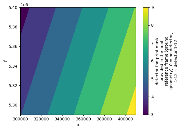

Selecting a Region and Verifying Detector Consistency¶

Wave spectrum analysis requires high resolution data. Thus we focus our analysis on 10 m spatial resolution band, such as B04 and B02, which are available in Sentinel-2 L1C products.

A 5 km × 5 km area of interest was manually selected using the UTM grid. To ensure accurate wave spectrum computation, we verify that the selected region in both bands corresponds to the same detector.

This verification step helps ensure consistency in viewing geometry. We also visualize the selected bands to inspect reflectance values before proceeding with spectral analysis.

Let’s first define the area and try to plot the area on the map

# Define patch size in meters
size = 5000  # in meter

# Ocean location example:
west_utm = 352_305
south_utm = 5_345_005

# Bounding box corners
east_utm = west_utm + size
north_utm = south_utm + size

# Draw UTM bounding box using HoloViews
box = hv.Rectangles([(west_utm, south_utm, east_utm, north_utm)]).opts(
    line_color="white", line_width=1, fill_alpha=0
)

print("Selected UTM coordinates:", west_utm, south_utm, east_utm, north_utm)

# Overlay selected region on RGB quicklook
l1c_plot * box

Loading...

Clipping the dataset¶

Let’s navigate to the 10 m spatial-resolution group at ["measurements"]["reflectance"]["r10m"], then clip the data to the bounding box defined above.

Once clipped, we name the 10 m resolution-band dataset r10m.

We will use this r10m dataset throughout the notebook.

Difference from SAFE workflow

For Level-1C and Level-2A, the granules, also called tiles, are 100x100km2 ortho-images in UTM(Universal Transverse Mercator) /WGS84 projection. The UTM In georeferenced north-up rasters the origin is the upper-left, so the vertical y coordinate in UTM grid is descending (values decrease downward). This is the usual convention for Sentinel-2 L1C SAFE products and is preserved in EOPF Zarr.

With xarray’s .sel, the slice order must match the coordinate order. On a descending y, thus a standard y=slice(south_utm, north_utm) returns an empty selection. Use one of the following instead:

method 1. Selecting the image with original descending y: y=slice(north_utm - 1, south_utm, 1)
- Other possible way of selecting data is specify the image location using ‘isel’, in this case .isel(y=slice(5000,5500))
method 2. Swap the selection of y with interval as -1, to have the image stored with (0,0) element correspoinding to lower-left (South West).: y=slice(south_utm, north_utm - 1, -1)

The original workflow were decoding the image in south to north (method 2). To aligne with the original SAFE workflow, we select the image here using y=slice(south_utm, north_utm - 1, -1)

When to call .persist()

At this stage, we may choose to call .persist() when creating r10m.
This tells Dask to load the data into distributed memory (across workers), which can significantly speed up repeated operations.

If we do not call .persist(), then each access will fetch the required chunks on demand.
Since we know that r10m will be accessed multiple times (for visualisation and numerical analysis), in this workflow it makes sense to call .persist() now.

By contrast, calling .load() loads the data into your local Jupyter process memory (not into the Dask workers). If your workflow does not rely on Dask, .load() may be more appropriate.

Use .persist() or .load() only when the clipped subset fits comfortably in memory.
If the dataset exceeds available memory, avoid persisting or loading to prevent exhausting your workers (with .persist()) or your Jupyter process (with .load()).

# Clip L1C to the box defined by west_utm/south_utm and east_utm/north_utm
# NOTE: y is descending (north-up), so we slice with a negative step.
l1c = l1c_original.sel(
    x=slice(west_utm, east_utm - 1), y=slice(south_utm, north_utm - 1, -1)
)

# Equivalent alternatives (kept here for reference):
# l1c = l1c_original.sel(x=slice(west_utm, east_utm - 1), y=slice(north_utm - 1, south_utm, 1))
# l1c = l1c_original.sel(x=slice(west_utm, east_utm - 1)).isel(y=slice(5000, 5500))

# Select the 10 m reflectance group as a Dataset, then persist if it fits in memory
r10m = l1c["measurements"]["reflectance"]["r10m"].to_dataset().persist()

# Quick sanity check with xarray’s Matplotlib integration
# r10m.b02.plot()

# (Optional) Compare array ordering with a raw Matplotlib image.
# Using .values forces a NumPy materialization; fine for small slices.
# plt.pcolormesh(r10m.b04.values, cmap="viridis"); plt.show()

Visualise all 10 m bands¶

We visualise here each variable in r10m using xarray’s hvplot integration. (All xarray objects expose a .hvplot accessor for easy plotting.)

Loop over r10m.data_vars and plot each band with hvplot using x="x" and y="y".
Set aspect="equal" so pixels are not distorted.
Set frame_width to control panel size, and switch colormaps via cmap.
Apply an ocean-themed, perceptually uniform colormap from cmocean (here cmocean.cm.ice) to keep patterns faithful while looking vibrant.
Arrange the individual plots into a simple grid layout with two columns.

plots = [
    r10m[var].hvplot(
        x="x",
        y="y",
        aspect="equal",  # keep pixel aspect ratio 1:1 (no geometric distortion)
        cmap=cmocean.cm.ice,  # Choose a perceptually uniform, ocean-themed sequential colormap from cmocean
        title=f"{var}",
        frame_width=200,  # thumbnail size; increase if you want larger panels
        # robust=True,           # auto color limits from 2nd–98th percentiles
        # clim=(vmin, vmax),     # define vmin and vmax then uncomment to enforce the same range across bands
        # rasterize=True,        # render via Datashader for large arrays (fast pan/zoom)
        # aggregator="min",      # optional: choose Datashader aggregator; default is usually 'mean'
    )
    for var in r10m.data_vars
]


# Layout plots horizontally, then display as two columns
layout = plots[0]
for p in plots[1:]:
    layout += p
layout.cols(2)

Loading...

Detector Consistency Verification¶

Sentinel-2 MSI imagery is collected by 12 detectors, each with slightly different viewing geometries.
For accurate wave spectral analysis, it is essential that our cropped region comes from a single detector to ensure:

Consistent viewing angles
Synchronized temporal sampling
Uniform spectral calibration

Here we check whether all pixels in the clipped region belong to the same detector.

# Extract detector IDs over the clipped area (cast to int for clarity).
# Persist so the array is kept in Dask memory for faster repeated access.
b04_detector = (
    l1c["conditions"]["mask"]["detector_footprint"]["r10m"]["b04"].astype(int).persist()
)

# Take the detector ID from the first pixel as a reference value.
detector = int(b04_detector.isel(y=0, x=0).compute())

# Check whether all detector IDs in the clipped region match the reference.
if bool((b04_detector == detector).all().compute()):
    print(f"✅ Single detector confirmed: {int(detector)}")
else:
    # If not unique, count how many pixels belong to each detector.
    counts = b04_detector.groupby(b04_detector).count().rename("count").compute()
    raise ValueError(f"b04_detector is not unique! : {counts}")

✅ Single detector confirmed: 6

Image Normalization and Whitecap Filtering¶

In this section, we normalize the bands and then apply an edge-based filter (Sobel + threshold) to reduce the influence of whitecaps (i.e., foam-related reflectance artefacts).

The original SAFE workflow used only two bands:

B04 (red)
B02 (blue)

With xarray, we can apply the same workflow in a simple and vectorised manner.
Thanks to the EOPF Zarr format, this functionality is available natively—no extra complexity—so let’s apply the operations to all r10m bands.

Median Normalization¶

We normalize each 10 m band in r10m by its spatial median (over x and y).
This centers reflectance around ~1.0 and makes bands comparable for later filtering and spectra—no axis transposition needed.

# Normalize by median
normalised_r10 = r10m.apply(
    lambda da: da / np.nanmedian(da.values),
)
normalised_r10 = normalised_r10.persist()

Sobel Filtering and Whitecap Masking¶

We apply a Sobel edge filter to each band to highlight intensity gradients (edges) typically associated with whitecaps or other strong reflectance structures, then mask pixels above each band’s 95th percentile gradient.

Using xarray keeps the pipeline lazy: Sobel is applied via apply(...), and thresholds use per-band quantile(0.95) so we avoid loading arrays eagerly.

# Apply the sobel operator
gradient_sobel = normalised_r10.apply(
    lambda da: sobel(da),
)
# gradient_sobel = gradient_sobel.persist() # we do not plot this value anywhere, so we keep it lazy (not compute here and triger the computation in later

# Threshold (95th percentile)
# Binary mask: retain only low-gradient (non-whitecap) regions
mask = gradient_sobel.apply(
    lambda da: da < np.percentile(da, 95),
)

# Apply mask: keep low-gradient (non-whitecap) pixels; drop high-gradient ones
filterd_r10m = (normalised_r10.where(mask, np.nan)).persist()
filterd_r10m

Loading...

# Plot the filtered image

plots = [
    filterd_r10m[var].hvplot(
        x="x",
        y="y",
        aspect="equal",
        # rasterize=True,
        cmap=cmocean.cm.ice,  # alternatives: cmocean.cm.deep, cmocean.cm.thermal
        clim=(0.9, 1.1),  # normalized reflectance ~1
        colorbar=True,
        clabel="Normalised Image",
        title=f"Filtered — {var}",
        frame_width=200,
    )
    for var in filterd_r10m.data_vars
]

# Layout plots horizontally
layout = plots[0]
for p in plots[1:]:
    layout += p

layout.cols(2)

Loading...

Pixel Value Distribution (Histogram)¶

We visualize the intensity distribution of the normalized reflectance values for bands using histograms. This step helps verify that the normalization behaves consistently across the two channels and that there are no outliers or saturation artifacts before spectral processing.

If it is a bimodial distribution, it may indicate the presense of clouds or other non wave related artifacts.

# Display the histogram of values for the original image

plots = [
    normalised_r10[var].hvplot.hist(
        bins=100,
        #    color='blue',
        alpha=0.3,
        xlabel="Pixel Value",
        ylabel="Frequency",
        title="Histogramme intensity of each bands",
        frame_width=400,
    )
    for var in filterd_r10m.data_vars
]
combined_reversed = plots[-1]
for p in plots[-2::-1]:
    combined_reversed = combined_reversed * p

combined_reversed

Loading...

Fourier Transform & Welch-Based Spectral Analysis¶

This section demonstrates a two-dimensional Fast Fourier Transform (FFT) analysis on paired Sentinel-2 images (e.g., bands B02 and B04). The core function, FFT2D_two_arrays_nonan, implements a Welch-style spectral estimate and is copy-pasted directly from the original research implementation.

What it does:

Image tiling: The images are partitioned into overlapping tiles controlled by ntile.
NaN handling: Within each tile, any NaNs (e.g., from filtering/masking) are replaced by the tile mean; tiles with >50% NaNs are skipped.
Windowing: A 2-D Hann (a.k.a. “Hanning”) window is applied per tile to reduce edge artefacts and spectral leakage.
FFT per tile: A 2-D FFT is computed for each windowed tile; power spectra are accumulated.
Welch averaging: Spectra across tiles are averaged to stabilise estimates and reduce noise.

Array orientation expected by the original function
FFT2D_two_arrays_nonan(arraya, arrayb, dx, dy, n, ...) expects NumPy arrays (arraya and arrayb) with the first dimension = x (west→east) and the second dimension = y (south→north).
EOPF Zarr exposes bands with dimensions ordered as (y, x), so we transpose to ("x","y") before calling the function.

Outputs

Eta, Etb: power spectral densities (PSDs) of each image
coh: spectral coherence between the two images
ang: phase difference (radians)
crosr: real part of the cross-spectrum
kx2, ky2: spatial frequency coordinates (cycles per metre)
dkxtile, dkytile: frequency resolution (x and y)

Reusing SAFE-era functions with EOPF Zarr

When calling Python code developed for SAFE inputs, be explicit about the array orientation that the function expects. Even though EOPF Zarr preserves the SAFE north-up storage, some SAFE workflows reordered arrays before analysis.

Once you’ve verified the expected order, reusing your function is straightforward: convert the xarray DataArray to a NumPy array in the right orientation, e.g.

arraya = filterd_r10m_transposed["b04"].compute().values

# Transpose Dataset so each band is (x, y) to match function expectations
# (EOPF Zarr typically exposes (y, x); we make it explicit here.)
filterd_r10m_transposed = filterd_r10m.transpose("x", "y")
filterd_r10m_transposed

Loading...

def FFT2D_two_arrays_nonan(arraya, arrayb, dx, dy, n, isplot=0):
    # Welch-based 2D spectral analysis
    # nxa, nya : size of arraya
    # dx, dy : resolution of arraya
    # n : number of tiles in each direction

    [nxa, nya] = np.shape(arraya)
    mspec = n**2 + (n - 1) ** 2
    nxtile = int(np.floor(nxa / n))
    nytile = int(np.floor(nya / n))

    dkxtile = 1 / (dx * nxtile)
    dkytile = 1 / (dy * nytile)

    shx = int(nxtile // 2)  # OK if nxtile is even number
    shy = int(nytile // 2)

    # --- Prepare wavenumber vectors ---
    kx = np.fft.fftshift(np.fft.fftfreq(nxtile, dx))
    ky = np.fft.fftshift(np.fft.fftfreq(nytile, dy))
    kx2, ky2 = np.meshgrid(kx, ky, indexing="ij")

    if isplot:
        X = np.arange(0, nxa * dx, dx)
        Y = np.arange(0, nya * dy, dy)

    # --- Prepare Hanning windows ---
    hanningx = 0.5 * (
        1 - np.cos(2 * np.pi * np.linspace(0, nxtile - 1, nxtile) / (nxtile - 1))
    )
    hanningy = 0.5 * (
        1 - np.cos(2 * np.pi * np.linspace(0, nytile - 1, nytile) / (nytile - 1))
    )
    hanningxy = np.atleast_2d(hanningy) * np.atleast_2d(hanningx).T

    wc2x = 1 / np.mean(hanningx**2)
    wc2y = 1 / np.mean(hanningy**2)
    normalization = (wc2x * wc2y) / (dkxtile * dkytile)

    # --- Initialize ---
    Eta = np.zeros((nxtile, nytile))
    Etb = np.zeros((nxtile, nytile))
    phase = np.zeros((nxtile, nytile), dtype=np.complex128)
    phases = np.zeros((nxtile, nytile, mspec), dtype=np.complex128)

    if isplot:
        fig1, ax1 = plt.subplots(figsize=(12, 6))
        ax1.pcolormesh(X, Y, arraya)
        # colors = plt.cm.seismic(np.linspace(0, 1, mspec))

    # --- Calculate spectrum for each tile ---
    nspec = 0
    for m in range(mspec):
        if m < n**2:
            i1 = int(np.floor(m / n) + 1)
            i2 = int(m + 1 - (i1 - 1) * n)

            ix1, ix2 = nxtile * (i1 - 1), nxtile * i1 - 1
            iy1, iy2 = nytile * (i2 - 1), nytile * i2 - 1
        else:
            i1 = int(np.floor((m - n**2) / (n - 1)) + 1)
            i2 = int(m + 1 - n**2 - (i1 - 1) * (n - 1))

            ix1, ix2 = nxtile * (i1 - 1) + shx, nxtile * i1 + shx - 1
            iy1, iy2 = nytile * (i2 - 1) + shy, nytile * i2 + shy - 1

        array1 = np.array(arraya[ix1 : ix2 + 1, iy1 : iy2 + 1], dtype=np.float64)
        array2 = np.array(arrayb[ix1 : ix2 + 1, iy1 : iy2 + 1], dtype=np.float64)

        # **Gestion des NaN**
        mask1 = np.isnan(array1)
        mask2 = np.isnan(array2)

        # Remplacement des NaN par la moyenne locale
        if np.any(mask1):
            array1[mask1] = np.nanmean(array1)
        if np.any(mask2):
            array2[mask2] = np.nanmean(array2)

        # Ignorer les tuiles avec trop de NaN (ex: >50% de la tuile)
        if np.sum(mask1) > 0.5 * array1.size or np.sum(mask2) > 0.5 * array2.size:
            continue

        # **Application de la fenêtre de Hanning en tenant compte des NaN**
        valid_mask1 = (~mask1).astype(float)
        valid_mask2 = (~mask2).astype(float)

        tile_centered = (array1 - np.nanmean(array1)) * valid_mask1
        tile_by_windows = tile_centered * hanningxy
        tileFFT1 = np.fft.fft2(tile_by_windows, norm="forward")
        tileFFT1_shift = np.fft.fftshift(tileFFT1)
        Eta += (abs(tileFFT1_shift) ** 2) * normalization

        tile_centered = (array2 - np.nanmean(array2)) * valid_mask2
        tile_by_windows = tile_centered * hanningxy
        tileFFT2 = np.fft.fft2(tile_by_windows, norm="forward")
        tileFFT2_shift = np.fft.fftshift(tileFFT2)
        Etb += (abs(tileFFT2_shift) ** 2) * normalization

        phase += tileFFT2_shift * np.conj(tileFFT1_shift) * normalization
        nspec += 1
        phases[:, :, m] = (
            tileFFT2_shift
            * np.conj(tileFFT1_shift)
            / (abs(tileFFT2_shift) * abs(tileFFT1_shift))
        )

    # **Rotation des phases autour de la moyenne**
    for m in range(mspec):
        phases[:, :, m] /= phase

    # **Normalisation finale**
    Eta /= nspec
    Etb /= nspec
    coh = abs((phase / nspec) ** 2) / (Eta * Etb)  # spectral coherence
    ang = np.angle(phase, deg=False)
    crosr = np.real(phase) / mspec
    angstd = np.std(np.angle(phases, deg=False), axis=2)

    return Eta, Etb, ang, angstd, coh, crosr, phases, kx2, ky2, dkxtile, dkytile


##############################################################################

# Pixel size in metres (Sentinel-2 10 m bands)
dx = dy = 10
ntile = 16
# Pass filtered images as NumPy arrays in (x, y) order
arraya = filterd_r10m_transposed["b04"].compute().values
arrayb = filterd_r10m_transposed["b02"].compute().values

(Eta, Etb, ang, angstd, coh, crosr, phases, kx2, ky2, dkx, dky) = (
    FFT2D_two_arrays_nonan(arraya, arrayb, dx, dy, ntile, isplot=0)
)

🌊 Fourier and Cross-Spectral Analysis with angular metrics.¶

With the Welch-based spectral analysis in place, the next step is to visualizes to analyzes spatial and spectral properties of satellite image data. To do so we need first to compute viewing geometry.

Computing Viewing Geometry : Sun and View Angles 🌞 📐¶

We want to extract sun and viewing angles from the Sentinel-2 L1C data product and compute relevant angular quantities such as phase angles or off-specular angles. These metrics help understand the scattering geometry at the selected region (e.g., for ocean wave analysis).

Accessing the Angle Data 🌞¶

The full datatree contains the geometry metadata at this location [‘conditions’][‘geometry’]: Angle layers may be provided at different native resolutions (e.g., r10m, r20m, r60m). We will visualise them and then sample the angles at the centre of our clipped region.

(
    l1c_original["conditions"]["geometry"]["sun_angles"].hvplot(
        x="x",
        y="y",
        aspect="equal",
        frame_width=200,
    )
    + l1c_original["conditions"]["geometry"]["viewing_incidence_angles"].hvplot(
        x="x",
        y="y",
        aspect="equal",
        frame_width=200,
    )
).cols(1)

Loading...

sun_angles = l1c["conditions"]["geometry"]["sun_angles"]
view_angles = l1c["conditions"]["geometry"]["viewing_incidence_angles"]
print("sun_angle:", sun_angles.compute().values)
print(
    "view_angle:",
    view_angles.sel(detector=detector, band=["b02", "b04"]).compute().values,
)

sun_angle: [[[ 27.0145]]

 [[152.472 ]]]
view_angle: [[[[ 1.13787]]

  [[89.3232 ]]]


 [[[ 1.38971]]

  [[67.2367 ]]]]

Since we’ve already clipped the image for our region of interest, we only extract the angles for this subset. However, the sampling grid might not be perfectly centered, so we need to interpolate the angle fields at the center of our clipped region.

The Center of the Clipped Region is:

x_val = (west_utm + east_utm) / 2
y_val = (south_utm + north_utm) / 2
print(x_val, y_val)

354805.0 5347505.0

But in our case, it is slightly be off the center of our image. So let’s get it interpolated.

Interpolating and Analyzing Viewing Geometry from Sentinel-2 L1C Data¶

To extract sun and viewing angles at a specific location in the scene, convert them to Cartesian unit vectors, and compute derived angular metrics for scattering geometry analysis.

Interpolating Angles at Arbitrary (x, y) Coordinates

def interpolate_angles_at_xy(x_val, y_val, angle_array):
    """
    Interpolate azimuth and zenith angles at (x, y) coordinates.

    Parameters:
        x_val (float): x coordinate
        y_val (float): y coordinate
        angle_array (xarray.DataArray): must have 'angle' dimension with 'zenith' and 'azimuth'

    Returns:
        xarray.DataArray: Interpolated angle array with dimensions (band, detector, angle)
    """
    angle_names = angle_array.angle.values
    if "azimuth" not in angle_names or "zenith" not in angle_names:
        raise ValueError("Missing 'azimuth' or 'zenith' in angle dimension.")

    zenith = angle_array.sel(angle="zenith").interp(x=x_val, y=y_val)
    azimuth = angle_array.sel(angle="azimuth")
    sin_az = np.sin(np.deg2rad(azimuth))
    cos_az = np.cos(np.deg2rad(azimuth))
    interp_sin = sin_az.interp(x=x_val, y=y_val)
    interp_cos = cos_az.interp(x=x_val, y=y_val)
    azimuth_corrected = (np.rad2deg(np.arctan2(interp_sin, interp_cos))) % 360

    result = xr.concat(
        [
            zenith.expand_dims(angle=["zenith"]),
            azimuth_corrected.expand_dims(angle=["azimuth"]),
        ],
        dim="angle",
    )
    return result


view_angles = interpolate_angles_at_xy(
    x_val, y_val, l1c_original["conditions"]["geometry"]["viewing_incidence_angles"]
)
sun_angles = interpolate_angles_at_xy(
    x_val, y_val, l1c_original["conditions"]["geometry"]["sun_angles"]
)
sun_angles.compute().values, view_angles.sel(
    detector=detector, band=["b02", "b04"]
).compute().values

(array([ 26.99460189, 152.45104   ]),
 array([[ 1.09648737,  1.35688407],
        [88.6205506 , 65.99286503]]))

Computes angular metrics comparable to the original Sentinel‑2 SAFE/SAFE2 XML‑based code, using Zarr format and xarray:¶

Spherical to Cartesian Conversion Convert interpolated zenith and azimuth angles (sun and view) into unit vectors: sunvec = sph2cart(sun_angles) and obsvec = sph2cart(view_angles).
Mid-Vector Calculation Sum and normalize the two direction vectors to obtain the mid-vector (midvec_norm) between sensor and sun hemispheres.
Derived Metrics Compute three angular metrics essential for scattering analysis:
- offspec: Off‑specular angle = angle between mid‑vector and vertical
- phitrig: Azimuth of mid‑vector (used to overlay blind azimuths on k‑space)
- thetav: Sensor view zenith angle
Selection for Specific Band & Detector Choose the relevant subset for a given detector and bands (e.g. B04 and B02):

def sph2cart(angle_da):
    """
    Convert spherical angles to Cartesian unit vectors.

    Parameters:
        angle_da (xarray.DataArray): must have 'angle' = ['zenith', 'azimuth']

    Returns:
        xarray.DataArray: shape (..., cartesian) with cartesian = ['x', 'y', 'z']
    """
    theta = np.radians(angle_da.sel(angle="zenith"))
    phi = np.radians(angle_da.sel(angle="azimuth"))
    x = np.sin(theta) * np.sin(phi)
    y = np.sin(theta) * np.cos(phi)
    z = np.cos(theta)
    return xr.concat([x, y, z], dim="cartesian").assign_coords(
        cartesian=["x", "y", "z"]
    )


# Compute Cartesian vectors
sunvec = sph2cart(sun_angles)
obsvec = sph2cart(view_angles)
# 🔄 Mid-Vector and Normalization
midvec = obsvec + sunvec
midvec_norm = midvec / np.sqrt((midvec**2).sum("cartesian"))
# 📐 Angular Metrics Computation
offspec = np.degrees(np.arccos(midvec_norm.sel(cartesian="z")))
phitrig = np.degrees(
    np.arctan2(midvec_norm.sel(cartesian="x"), midvec_norm.sel(cartesian="y"))
)
thetav = np.degrees(np.arccos(obsvec.sel(cartesian="z")))
phitrig = phitrig.sel(detector=6, band=["b04", "b02"]).compute()
phitrig

Loading...

This section overlays directional markers in Fourier space (k‑space) to emphasize blind azimuth angles—directions in which specular reflection (sunglint) is minimized. These are useful for interpreting wave fields in optical imagery, especially when bright reflections mask fine patterns.

Waves propagating along these blind directions are expected to produce minimal brightness modulation due to the geometry of sun-sensor alignment, making them harder to detect.

To compute and overlay these directions:

phitrig[b] is the azimuth angle (in degrees) of the mid-vector between the sun and sensor directions, previously computed for each band b.
The blind azimuth direction is calculated as:
```
phiblind = phitrig + 90
```
This is orthogonal to the mid-vector, i.e., the direction where sunglint is minimized.
k-space overlay vectors are then defined as:
```
±1.4 * kN * [sin(phiblind), cos(phiblind)]  
```
where:
- kN = 50 is a manual scaling factor to make the vectors visually prominent in spectral plots.
- The ± sign draws symmetric vectors in both directions.

These vectors are plotted as dashed lines on 2D spectral maps (e.g., power, coherence, phase) to visualize and assess whether wave energy aligns with or avoids these blind azimuth directions.

This visualization is especially helpful to confirm directional biases in wave energy related to illumination and viewing geometry.

# Compute blind azimuth:
phiblind1 = phitrig[0].values + 90.0  # blind azimuth for B04
phiblind2 = phitrig[1].values + 90.0  # blind azimuth for B02
kN = 50
xkblind = [
    -1.4 * kN * np.sin(np.radians(phiblind1)),
    1.4 * kN * np.sin(np.radians(phiblind2)),
]
ykblind = [
    -1.4 * kN * np.cos(np.radians(phiblind1)),
    1.4 * kN * np.cos(np.radians(phiblind2)),
]
print(xkblind, ykblind)

[60.30159381316901, -60.81853346026498] [35.54880846936472, -34.65697603286573]

Physical Interpretation of Results¶

Let’s analyse the result of Fourier and Cross-Spectral with angular metrics and understand the result.

We will first compute Variance and Energy Check, then make 4 different set of plots and make interpretation.

0. 🧮 Variance and Energy Check¶

Compares spatial domain variance to spectral energy.
A consistency check based on Parseval’s theorem.

# Parseval/variance checks
print("variance B04:", np.nanvar(arraya), "sum of spectrum:", np.sum(Eta) * dkx * dky)
print("variance B02:", np.nanvar(arrayb), "sum of spectrum:", np.sum(Etb) * dkx * dky)

variance B04: 0.004539154168472143 sum of spectrum: 0.003969145049406069
variance B02: 0.0006660525439104757 sum of spectrum: 0.0005955796139226746

1. 🖼️ Surface Image Plot¶

What we see: Filtered Sentinel-2 B04 reflectance showing ocean wave patterns
Preprocessing: Whitecaps removed, median normalized, edge effects minimized
Scale: 5×5 km region with 10m pixel resolution
Pattern: Clear wave trains visible as brightness variations

# 1) Surface image (B04)

# Grid from the filtered dataset
(ny, nx) = filterd_r10m["b04"].shape
X = np.arange(0, nx * dx, dx)  # [m]
Y = np.arange(0, ny * dy, dy)

fig, ax = plt.subplots(figsize=(10, 5))
ax.set_aspect("equal", adjustable="box")
im = ax.pcolormesh(
    X / 1000,
    Y / 1000,
    filterd_r10m["b04"].values,
    cmap="seismic",
    norm=mcolors.Normalize(vmin=0.5, vmax=2),
)
plt.colorbar(im, ax=ax, label="S2 image band B04")
ax.set_xlabel("X [km]")
ax.set_ylabel("Y [km]")
ax.set_title("Surface")
plt.tight_layout()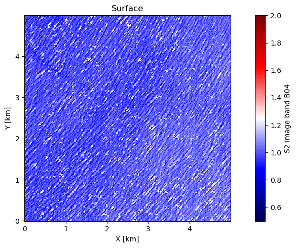

2. 📊 Power Spectrum Plot¶

What we see: 2D Fourier transform revealing dominant wave directions
Axes: Spatial frequency (cycles/km) in X and Y directions
Interpretation:
- Bright regions = dominant wave energy
- Peak locations = wavelength and direction
- Dashed line = satellite viewing geometry (blind direction)
Key Finding: Energy concentrated in NW-SE direction, indicating swell propagation

# 2) Spectrum (Eta) in dB
fig, ax = plt.subplots(figsize=(10, 5))
ax.set_aspect("equal", adjustable="box")
im = ax.pcolormesh(
    kx2 * 1000,
    ky2 * 1000,
    10 * np.log10(Eta),
    norm=mcolors.Normalize(vmin=-30, vmax=20),
)
plt.colorbar(im, ax=ax, label="dB")
ax.plot(xkblind, ykblind, color="k", linestyle="--", linewidth=2)
ax.set_xlabel("k_x [cycles / km]")
ax.set_ylabel("k_y [cycles / km]")
ax.set_title("Spectrum")
plt.tight_layout()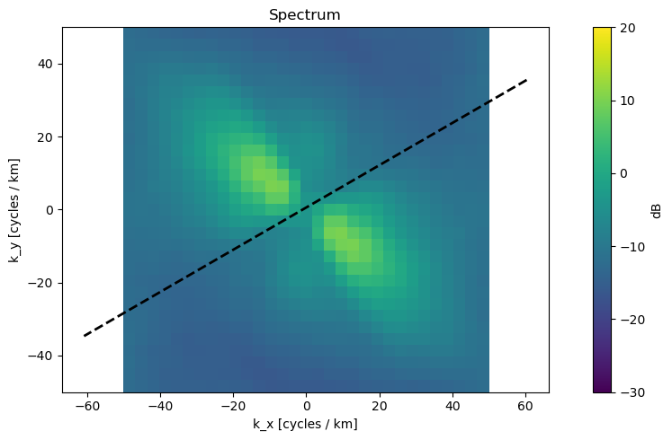

3. 🔗 Coherence Map¶

What we see: Correlation between B02 and B04 bands in frequency space
Values: 0 (random noise) to 1 (perfect correlation)
Interpretation:
- High coherence (yellow) = real wave signals
- Low coherence (blue) = instrumental noise or artifacts
Quality Metric: Coherence >0.7 indicates reliable wave measurements

# 3-1) Coherence
fig, ax = plt.subplots(figsize=(10, 5))
ax.set_aspect("equal", adjustable="box")
im = ax.pcolormesh(
    kx2 * 1000,
    ky2 * 1000,
    coh,
    norm=mcolors.Normalize(vmin=0, vmax=1),
)
plt.colorbar(im, ax=ax, label=" ")
ax.plot(xkblind, ykblind, color="k", linestyle="--", linewidth=2)
ax.set_xlabel("k_x [cycles / km]")
ax.set_ylabel("k_y [cycles / km]")
ax.set_title("Coherence B02–B04")
plt.tight_layout()

# 3-2) Coherence (rad/m axes)
# convert xkblind, ykblind from cycles/km  → rad/m
def to_radm(seq):
    fact = 2 * np.pi / 1000.0
    if (
        isinstance(seq, (list, tuple))
        and len(seq) > 0
        and isinstance(seq[0], (list, tuple, np.ndarray))
    ):
        return [np.asarray(s, dtype=float) * fact for s in seq]
    return np.asarray(seq, dtype=float) * fact


xkblind_radm = to_radm(xkblind)
ykblind_radm = to_radm(ykblind)


fig, ax = plt.subplots(figsize=(10, 5))
ax.set_aspect("equal", adjustable="box")
im = ax.pcolormesh(
    kx2 * 2 * np.pi,
    ky2 * 2 * np.pi,
    coh,
    norm=mcolors.Normalize(vmin=0, vmax=1),
)
plt.colorbar(im, ax=ax, label=" ")
ax.plot(xkblind_radm, ykblind_radm, color="k", linestyle="--", linewidth=2)

ax.set_xlabel("k_x [rad / m]")
ax.set_ylabel("k_y [rad / m]")
ax.set_title("Coherence B02–B04")
plt.tight_layout()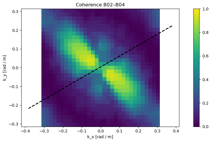

4. 🔄 Cross-Spectrum Phase Difference¶

This Cross-Spectrum is using the time lag between B02 and B04 acquisitions.

What we see: Phase angle of the cross-spectrum between two bands. Indicates relative shifts between features in different spectral bands.
Physical Meaning: Wave propagation direction and speed
Color Scale: ±180 degrees phase difference
Key Insight:
- Positive phase (red) in NW quadrant
- Negative phase (blue) in SE quadrant
- **Indicates waves moving from NW to SE during 1-second B02-B04 delay **

# 4) Cross-spectrum phase (degrees)
fig, ax = plt.subplots(figsize=(10, 7))
ax.set_aspect("equal", adjustable="box")
im = ax.pcolormesh(
    kx2 * 1000,
    ky2 * 1000,
    np.degrees(ang),
    cmap="seismic",
    norm=mcolors.Normalize(vmin=-180, vmax=180),
)
plt.colorbar(im, ax=ax, label="degrees")
ax.plot(xkblind, ykblind, color="k", linestyle="--", linewidth=2)
ax.set_xlabel("k_x [cycles / km]")
ax.set_ylabel("k_y [cycles / km]")
ax.set_title("Cross-spectrum phase")
plt.tight_layout()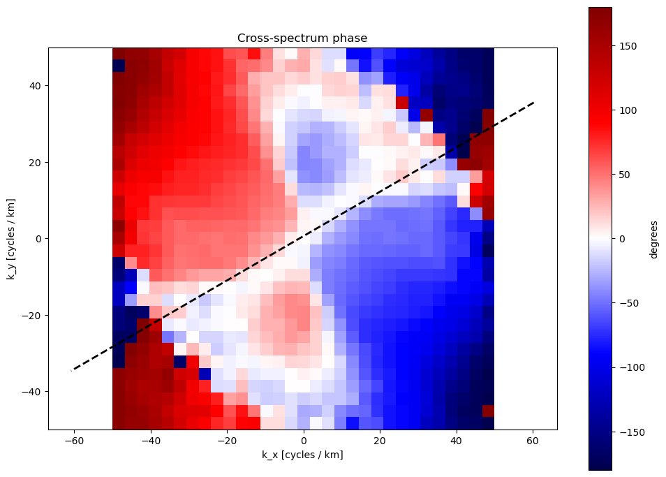

Scientific Significance¶

This analysis reveals:

Wave Direction: NW-SE propagation consistent with Atlantic swell patterns
Wave Quality: High coherence confirms reliable measurements using EOPF datasets
Propagation Speed: Phase gradient indicates ~15-20 m/s wave celerity
Methodology Validation: Results consistent with expected oceanographic conditions published in the Bay of Biscay (See Link to the WW3 simulation website).

Summary¶

This script performs comprehensive spectral analysis of satellite imagery by:

Visualizing filtered spatial data
Computing 2D Fourier spectra
Quantifying inter-band similarity via coherence and cross-spectral phase
Evaluating energy consistency between spatial and spectral domains

It is especially useful in oceanographic but also Earth surface pattern studies (e.g., wave fields, vegetation patterns, surface roughness).

Transforming workflow for oceanography study using Sentinel‑2 data, from SAFE to Zarr

Table of contents¶

Introduction¶

Setup and Dependencies¶

Accessing Sentinel-2 Data in EOPF Zarr Format via STAC¶

Loading Sentinel-2 Data with xarray (EOPF Zarr)¶

Opening Sentinel-2 L1C as a Datatree¶

Detector Identification¶

Selecting a Region and Verifying Detector Consistency¶

Clipping the dataset¶

Visualise all 10 m bands¶

Detector Consistency Verification¶

Image Normalization and Whitecap Filtering¶

Median Normalization¶

Sobel Filtering and Whitecap Masking¶

Pixel Value Distribution (Histogram)¶

Fourier Transform & Welch-Based Spectral Analysis¶

🌊 Fourier and Cross-Spectral Analysis with angular metrics.¶

Computing Viewing Geometry : Sun and View Angles 🌞 📐¶

Accessing the Angle Data 🌞¶

Interpolating and Analyzing Viewing Geometry from Sentinel-2 L1C Data¶

Computes angular metrics comparable to the original Sentinel‑2 SAFE/SAFE2 XML‑based code, using Zarr format and xarray:¶

Blind Azimuth Vectors in Fourier Space¶

Physical Interpretation of Results¶

0. 🧮 Variance and Energy Check¶

1. 🖼️ Surface Image Plot¶

2. 📊 Power Spectrum Plot¶

3. 🔗 Coherence Map¶

4. 🔄 Cross-Spectrum Phase Difference¶

Scientific Significance¶

Summary¶