xarray EOPF backend - Sentinel-3 Native Mode

Table of Contents¶

Introduction
Import modules
Open a Sentinel-3 OLCI L1 EFR
Open a Sentinel-3 OLCI L1 ERR
Open a Sentinel-3 SLSTR Level-2 LST
Conclusion

Run this notebook interactively with all dependencies pre-installed

Introduction¶

xarray-eopf is a Python package that extends xarray with a custom backend called "eopf-zarr". This backend enables seamless access to ESA EOPF data products stored in the Zarr format, presenting them as analysis-ready data structures.

In this notebook, we demonstrate how to use the xarray-eopf backend to access Sentinel-3 EOPF Zarr products in native mode. All data access is lazy, meaning that data is only loaded when required—for example, during plotting or when writing to storage.

For a general introduction to the xarray EOPF backend, see the introduction notebook.

🐙 GitHub: EOPF Sample Service – xarray-eopf
❗ Issue Tracker: Submit or view issues
📘 Documentation: xarray-eopf Docs

Import Modules¶

The xarray-eopf backend is implemented as a plugin for xarray. Once installed, it registers automatically and requires no additional import. You can simply import xarray as usual:

import datetime

import matplotlib.pyplot as plt
import pystac_client
import xarray as xr

Open a Sentinel-3 OLCI L1 EFR¶

We begin with an example that accesses a Sentinel-3 OLCI L1 EFR product in native mode.

Find a Sentinel-3 OLCI L1 EFR Zarr Sample via STAC¶

To obtain a product URL, you can use the STAC Browser to search for a Sentinel-3 OLCI Level-1 EFR tile.

catalog = pystac_client.Client.open("https://stac.core.eopf.eodc.eu")
items = list(
    catalog.search(
        collections=["sentinel-3-olci-l1-efr"],
        bbox=[7.2, 44.5, 7.4, 44.7],
        datetime=[str(datetime.date.today() - datetime.timedelta(days=5)), None],
    ).items()
)
items

[<Item id=S3B_OL_1_EFR____20260329T094553_20260329T094853_20260329T114455_0179_118_193_2160_ESA_O_NR_004>,
 <Item id=S3B_OL_1_EFR____20260328T101204_20260328T101504_20260328T121637_0179_118_179_2160_ESA_O_NR_004>,
 <Item id=S3B_OL_1_EFR____20260328T101204_20260328T101504_20260329T100706_0180_118_179_2160_ESA_O_NT_004>,
 <Item id=S3A_OL_1_EFR____20260327T093557_20260327T093857_20260328T103721_0179_137_307_2160_PS1_O_NT_004>,
 <Item id=S3A_OL_1_EFR____20260327T093557_20260327T093857_20260327T113653_0180_137_307_2160_PS1_O_NR_004>,
 <Item id=S3A_OL_1_EFR____20260326T100207_20260326T100507_20260327T110434_0180_137_293_2160_PS1_O_NT_004>,
 <Item id=S3A_OL_1_EFR____20260326T100207_20260326T100507_20260326T120302_0179_137_293_2160_PS1_O_NR_004>,
 <Item id=S3B_OL_1_EFR____20260326T092326_20260326T092626_20260327T093749_0179_118_150_2160_ESA_O_NT_004>,
 <Item id=S3B_OL_1_EFR____20260326T092326_20260326T092626_20260326T113241_0179_118_150_2160_ESA_O_NR_004>,
 <Item id=S3B_OL_1_EFR____20260325T094937_20260325T095237_20260326T102555_0179_118_136_2160_ESA_O_NT_004>,
 <Item id=S3B_OL_1_EFR____20260325T094937_20260325T095237_20260325T125634_0179_118_136_2160_ESA_O_NR_004>]

Next, we can inspect the item’s contents. The asset "product" links to the entire Zarr store. The additional field xarray:open_datatree_kwargs has been included in the asset "product", which provides the arguments needed to open the product using Xarray’s eopf-zarr engine.

item = items[1]
item

Open Sentinel-3 OLCI L1 EFR as DataTree¶

We can use the "product" asset to obtain the href and xarray:open_datatree_kwargs from the STAC item, and open the product as an xarray.DataTree as shown below:

dt = xr.open_datatree(
    item.assets["product"].href,
    **item.assets["product"].extra_fields["xarray:open_datatree_kwargs"],
)
dt

As an example, we plot the red band (oa08_radiance), which will trigger loading and visualization of the data. We also plot the 2D curvilinear latitude and longitude grids, which can be used for geolocation.

Note: To speed up rendering of large datasets in Matplotlib, we plot the data at a lower resolution (every 4th pixel).

fig, ax = plt.subplots(1, 3, figsize=(15, 4))
dt.measurements.oa08_radiance[::4, ::4].plot.imshow(ax=ax[0], vmin=0, vmax=300)
dt.measurements.latitude[::4, ::4].plot.imshow(ax=ax[1], cmap="viridis")
dt.measurements.longitude[::4, ::4].plot.imshow(ax=ax[2], cmap="viridis")
plt.tight_layout()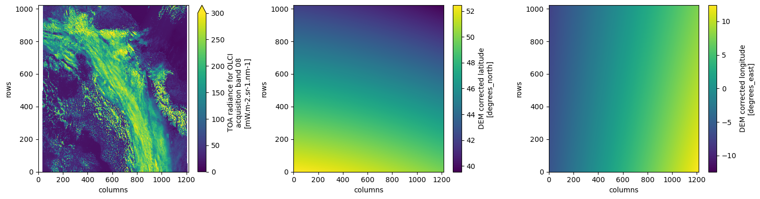

Open Sentinel-3 OLCI L1 EFR Radiance Group as Dataset¶

We can directly access the individual reflectance group (radianceData) as xarray.Dataset objects. The opening parameters are stored in the asset’s extra field "xarray:open_dataset_kwargs".

ds = xr.open_dataset(
    item.assets["radianceData"].href,
    **item.assets["radianceData"].extra_fields["xarray:open_dataset_kwargs"],
)
ds

We can also filter the varaibles by band names as shown below:

ds = xr.open_dataset(
    item.assets["radianceData"].href,
    **item.assets["radianceData"].extra_fields["xarray:open_dataset_kwargs"],
    variables="oa0[468]",
)
ds

And we can again plot the red band, which triggers loading the data.

ds.oa08_radiance[::4, ::4].plot(vmax=300)

Open Sentinel-3 OLCI L1 EFR as Dataset¶

The xarray.DataTree model was introduced in xarray v2024.10.0 (October 2024). To maintain compatibility with workflows based on xr.Dataset, the function xarray.open_dataset(..., engine="eopf-zarr", op_mode="native") is provided, which flattens the DataTree into a single dataset.

During this process, hierarchical groups in the Zarr product are merged, and variable as well as dimension names are prefixed with their group paths (using _ by default) to ensure uniqueness. For example, measurements/oa08_radiance becomes measurements_oa08_radiance.

ds = xr.open_dataset(
    item.assets["product"].href,
    engine="eopf-zarr",
    op_mode="native",
    chunks={},
)
ds

The separator character used in flattened variable names can be customized via the group_sep parameter. Additionally, you can filter the returned variables using the variables keyword argument, which accepts a string, an iterable of names, or a regular expression (regex) pattern.

ds = xr.open_dataset(
    item.assets["product"].href,
    engine="eopf-zarr",
    op_mode="native",
    chunks={},
    group_sep="/",
    variables="measurements*.",
)
ds

Also here, we can plot one spectral band as an example.

ds["measurements/oa08_radiance"][::4, ::4].plot(vmin=0.0, vmax=300.0)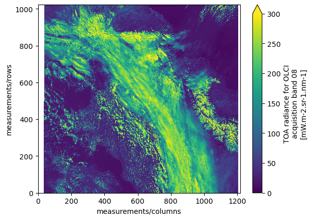

Open a Sentinel-3 OLCI L1 ERR¶

We now access a Sentinel-3 OLCI L1 ERR product in native mode. The data access methods shown above apply equally to Sentinel-3 OLCI L1 EFR.

Find a Sentinel-3 OLCI L1 ERR Zarr Sample via STAC¶

To obtain a product URL, you can use the STAC Browser to search for available Sentinel-3 OLCI L1 ERR tiles.

catalog = pystac_client.Client.open("https://stac.core.eopf.eodc.eu")
items = list(
    catalog.search(
        collections=["sentinel-3-olci-l1-err"],
        bbox=[7.2, 44.5, 7.4, 44.7],
        datetime=[str(datetime.date.today() - datetime.timedelta(days=5)), None],
    ).items()
)
items

[<Item id=S3B_OL_1_ERR____20260329T093543_20260329T101948_20260329T120344_2645_118_193______ESA_O_NR_004>,
 <Item id=S3B_OL_1_ERR____20260328T100201_20260328T104605_20260329T095351_2644_118_179______ESA_O_NT_004>,
 <Item id=S3B_OL_1_ERR____20260328T100201_20260328T104605_20260328T122605_2644_118_179______ESA_O_NR_004>,
 <Item id=S3A_OL_1_ERR____20260327T092601_20260327T101004_20260328T103618_2643_137_307______PS1_O_NT_004>,
 <Item id=S3A_OL_1_ERR____20260327T092601_20260327T101004_20260327T113524_2643_137_307______PS1_O_NR_004>,
 <Item id=S3A_OL_1_ERR____20260326T095219_20260326T103622_20260327T110333_2643_137_293______PS1_O_NT_004>,
 <Item id=S3A_OL_1_ERR____20260326T095219_20260326T103622_20260326T120200_2643_137_293______PS1_O_NR_004>,
 <Item id=S3B_OL_1_ERR____20260326T091338_20260326T095741_20260327T092230_2643_118_150______ESA_O_NT_004>,
 <Item id=S3B_OL_1_ERR____20260326T091338_20260326T095741_20260326T114137_2643_118_150______ESA_O_NR_004>,
 <Item id=S3B_OL_1_ERR____20260325T093956_20260325T102359_20260326T101436_2643_118_136______ESA_O_NT_004>,
 <Item id=S3B_OL_1_ERR____20260325T093956_20260325T102359_20260325T120957_2643_118_136______ESA_O_NR_004>]

item = items[0]
item

Open Sentinel-3 OLCI L1 ERR as DataTree¶

We can use the "product" asset to obtain the href and xarray:open_datatree_kwargs from the STAC item, and open the product as an xarray.DataTree as shown below:

dt = xr.open_datatree(
    item.assets["product"].href,
    **item.assets["product"].extra_fields["xarray:open_datatree_kwargs"],
)
dt

Open Sentinel-3 OLCI L1 EFF Radiance Group as Dataset¶

We can directly access the individual reflectance group (radianceData) as xarray.Dataset objects. The opening parameters are stored in the asset’s extra field "xarray:open_dataset_kwargs".

ds = xr.open_dataset(
    item.assets["radianceData"].href,
    **item.assets["radianceData"].extra_fields["xarray:open_dataset_kwargs"],
)
ds

Note: To speed up rendering of large datasets in Matplotlib, we plot the data at a lower resolution (every 4th pixel along-track).

fig, ax = plt.subplots(1, 3, figsize=(10, 5))
ds.oa08_radiance[::4, :].plot.imshow(ax=ax[0], vmin=0, vmax=300)
ds.latitude[::4, :].plot.imshow(ax=ax[1], cmap="viridis")
ds.longitude[::4, :].plot.imshow(ax=ax[2], cmap="viridis")
plt.tight_layout()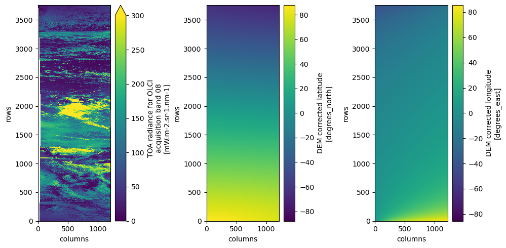

Open a Sentinel-3 SLSTR Level-2 LST¶

We now access a Sentinel-3 SLSTR Level-2 LST product in native mode. The data access methods shown above apply equally to Sentinel-3 SLSTR Level-2 LST.

Find a Sentinel-3 SLSTR Level-2 LST Zarr Sample via STAC¶

To obtain a product URL, you can use the STAC Browser to search for a Sentinel-3 SLSTR Level-2 LST tile.

catalog = pystac_client.Client.open("https://stac.core.eopf.eodc.eu")
items = list(
    catalog.search(
        collections=["sentinel-3-slstr-l2-lst"],
        bbox=[7.2, 44.5, 7.4, 44.7],
        datetime=[str(datetime.date.today() - datetime.timedelta(days=5)), None],
    ).items()
)
items

[<Item id=S3A_SL_2_LST____20260329T214729_20260329T215029_20260330T003114_0179_137_343_0720_PS1_O_NR_004>,
 <Item id=S3B_SL_2_LST____20260329T210848_20260329T211148_20260329T235533_0179_118_200_0720_ESA_O_NR_004>,
 <Item id=S3A_SL_2_LST____20260329T102435_20260329T102735_20260329T125030_0179_137_336_2160_PS1_O_NR_004>,
 <Item id=S3B_SL_2_LST____20260329T094553_20260329T094853_20260329T121220_0179_118_193_2160_ESA_O_NR_004>,
 <Item id=S3B_SL_2_LST____20260328T213459_20260328T213759_20260329T001031_0179_118_186_0720_ESA_O_NR_004>,
 <Item id=S3B_SL_2_LST____20260328T213459_20260328T213759_20260330T051647_0179_118_186_0720_ESA_O_NT_004>,
 <Item id=S3A_SL_2_LST____20260328T203241_20260328T203541_20260328T231506_0179_137_328_0720_PS1_O_NR_004>,
 <Item id=S3A_SL_2_LST____20260328T203241_20260328T203541_20260330T081257_0179_137_328_0720_PS1_O_NT_004>,
 <Item id=S3B_SL_2_LST____20260328T101204_20260328T101504_20260328T123424_0179_118_179_2160_ESA_O_NR_004>,
 <Item id=S3B_SL_2_LST____20260328T101204_20260328T101504_20260329T172450_0180_118_179_2160_ESA_O_NT_004>,
 <Item id=S3A_SL_2_LST____20260327T205851_20260327T210151_20260329T083311_0179_137_314_0720_PS1_O_NT_004>,
 <Item id=S3A_SL_2_LST____20260327T205851_20260327T210151_20260327T234107_0179_137_314_0720_PS1_O_NR_004>,
 <Item id=S3A_SL_2_LST____20260327T093557_20260327T093857_20260328T204053_0179_137_307_2160_PS1_O_NT_004>,
 <Item id=S3A_SL_2_LST____20260327T093557_20260327T093857_20260327T120121_0180_137_307_2160_PS1_O_NR_004>,
 <Item id=S3A_SL_2_LST____20260326T212502_20260326T212802_20260328T091525_0179_137_300_0720_PS1_O_NT_004>,
 <Item id=S3A_SL_2_LST____20260326T212502_20260326T212802_20260327T000636_0179_137_300_0720_PS1_O_NR_004>,
 <Item id=S3B_SL_2_LST____20260326T204621_20260326T204921_20260328T030457_0179_118_157_0720_ESA_O_NT_004>,
 <Item id=S3B_SL_2_LST____20260326T204621_20260326T204921_20260326T232930_0180_118_157_0720_ESA_O_NR_004>,
 <Item id=S3A_SL_2_LST____20260326T100207_20260326T100507_20260327T212028_0180_137_293_2160_PS1_O_NT_004>,
 <Item id=S3A_SL_2_LST____20260326T100207_20260326T100507_20260326T122451_0179_137_293_2160_PS1_O_NR_004>,
 <Item id=S3B_SL_2_LST____20260326T092326_20260326T092626_20260327T153634_0179_118_150_2160_ESA_O_NT_004>,
 <Item id=S3B_SL_2_LST____20260326T092326_20260326T092626_20260326T114832_0179_118_150_2160_ESA_O_NR_004>,
 <Item id=S3B_SL_2_LST____20260325T211231_20260325T211531_20260327T033756_0179_118_143_0720_ESA_O_NT_004>,
 <Item id=S3B_SL_2_LST____20260325T211231_20260325T211531_20260325T234726_0179_118_143_0720_ESA_O_NR_004>,
 <Item id=S3A_SL_2_LST____20260325T102818_20260325T103118_20260326T221710_0180_137_279_2160_PS1_O_NT_004>,
 <Item id=S3A_SL_2_LST____20260325T102818_20260325T103118_20260325T125251_0180_137_279_2160_PS1_O_NR_004>,
 <Item id=S3B_SL_2_LST____20260325T094937_20260325T095237_20260326T161103_0179_118_136_2160_ESA_O_NT_004>,
 <Item id=S3B_SL_2_LST____20260325T094937_20260325T095237_20260325T122544_0179_118_136_2160_ESA_O_NR_004>]

item = items[0]
item

Open Sentinel-3 SLSTR Level-2 LST as DataTree¶

We can use the "product" asset to obtain the href and xarray:open_datatree_kwargs from the STAC item, and open the product as an xarray.DataTree as shown below:

dt = xr.open_datatree(
    item.assets["product"].href,
    **item.assets["product"].extra_fields["xarray:open_datatree_kwargs"],
)
dt

Open Sentinel-3 SLSTR Level-2 LST Group as Dataset¶

Similarly, we can directly access the individual LST group (lst) as xarray.Dataset objects.

ds = xr.open_dataset(
    item.assets["lst"].href, engine="eopf-zarr", op_mode="native", chunks={}
)
ds

And we can plot the LST array along with the 2D latitude and longitude grids.

fig, ax = plt.subplots(1, 3, figsize=(15, 4))
ds.lst.plot.imshow(ax=ax[0])
ds.latitude.plot.imshow(ax=ax[1], cmap="viridis")
ds.longitude.plot.imshow(ax=ax[2], cmap="viridis")
plt.tight_layout()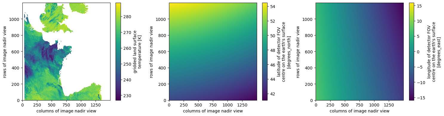

Other Sentinel-3 products can be accessed using the same approach and are therefore not shown here in detail.

Conclusion¶

This notebook demonstrates how to access Sentinel-3 EOPF Zarr samples in native mode using the xarray-eopf plugin. Key takeaways are:

Access all Sentinel-3 products using hte same methods.
Open the full Zarr store as an xr.DataTree using xr.open_dataset and the asset "product".
Open subgroups (e.g., radianceData, lst) as xr.Dataset using xr.open_dataset.
Open the full Zarr store as a flattened xr.Dataset using xr.open_dataset and the asset "product".
Filter variables using the variables keyword argument.
Opening parameters are integrated in STAC assets.

Note: This notebook only covers the native mode, which presents the data as close as possible to the original product.
For an analysis-ready view, see the Sentinel-3 analysis mode notebook.