Sentinel-1 GRD Geolocation with EOPFZARR Driver
Ground Control Point (GCP) based geolocation for Sentinel-1 GRD products using the EOPFZARR GDAL driver

Sentinel-1 GRD Geolocation with EOPFZARR Driver
Run this notebook interactively with all dependencies pre-installed
Table of Contents
Introduction
Sentinel-1 GRD (Ground Range Detected) products use Ground Control Points (GCPs) for geolocation — a sparse grid of pixel/line → longitude/latitude/height correspondences stored in conditions/gcp/ arrays.
Unlike optical sensors (Sentinel-2/3) that use dense coordinate arrays or affine geotransforms, Sentinel-1 uses a sparse grid of Ground Control Points stored in conditions/gcp/:
pixel(1D) andline(1D) define the image grid positionslatitude(2D),longitude(2D),height(2D) define the geographic positions
The EOPFZARR driver automatically reads these arrays and attaches them as GDAL GCPs to measurement subdatasets, enabling reprojection and coordinate transformation.
Setup
import numpy as np
import matplotlib.pyplot as plt
from osgeo import gdal, osr

gdal.UseExceptions()

print(f"GDAL version: {gdal.__version__}")

drv = gdal.GetDriverByName("EOPFZARR")
if drv:
    print("EOPFZARR driver: Registered")
else:
    print("WARNING: EOPFZARR driver not found!")
GDAL version: 3.12.0dev-209c099c56
EOPFZARR driver: Registered
Dataset Configuration
We use a Sentinel-1C IW mode GRD product with dual VV/VH polarization.
GRD_URL = (
    "/vsicurl/https://objects.eodc.eu/e05ab01a9d56408d82ac32d69a5aae2a:"
    "notebook-data/tutorial_data/cpm_v264/"
    "S1C_IW_GRDH_1SDV_20260205T120122_20260205T120158_006220_00C7E4_5D6E.zarr"
)

zarr_path = f"EOPFZARR:'{GRD_URL}'"

print("Dataset: S1C_IW_GRDH_1SDV")
print("  Platform:      Sentinel-1C")
print("  Mode:          IW (Interferometric Wide)")
print("  Resolution:    High")
print("  Polarization:  Dual VV/VH")
Dataset: S1C_IW_GRDH_1SDV
Platform: Sentinel-1C
Mode: IW (Interferometric Wide)
Resolution: High
Polarization: Dual VV/VH
Open a GRD Subdataset
We open the product with GRD_MULTIBAND=NO to access individual subdatasets, then open the VV measurement. GCPs are automatically attached to each measurement subdataset.
# Open product in standard mode to see subdatasets
root_ds = gdal.OpenEx(zarr_path, gdal.OF_RASTER, open_options=["GRD_MULTIBAND=NO"])

subdatasets = root_ds.GetMetadata("SUBDATASETS")

# Find the VV GRD measurement subdataset
vv_path = None
for key, value in sorted(subdatasets.items()):
    if "_NAME" in key and "measurements/grd" in value and "_VV" in value:
        vv_path = value
        break

print(f"VV subdataset: {vv_path.split(':/')[1] if vv_path else 'not found'}")

# Open the VV subdataset
ds = gdal.Open(vv_path)
print(f"\nDimensions: {ds.RasterXSize} x {ds.RasterYSize} pixels")
print(f"Data Type:  {gdal.GetDataTypeName(ds.GetRasterBand(1).DataType)}")

root_ds = None
VV subdataset: /objects.eodc.eu/e05ab01a9d56408d82ac32d69a5aae2a:notebook-data/tutorial_data/cpm_v264/S1C_IW_GRDH_1SDV_20260205T120122_20260205T120158_006220_00C7E4_5D6E.zarr"
Dimensions: 25157 x 24285 pixels
Data Type: UInt16
Inspect GCPs
The driver automatically extracts GCPs from the conditions/gcp/ arrays and attaches them to the dataset.
gcp_count = ds.GetGCPCount()
print(f"GCP Count: {gcp_count}")

# Check the GCP spatial reference
gcp_srs = ds.GetGCPSpatialRef()
if gcp_srs:
    print(f"GCP SRS:   {gcp_srs.GetName()} (EPSG:{gcp_srs.GetAuthorityCode(None)})")

# Display the GCPs
gcps = ds.GetGCPs()
print("\nFirst 10 GCPs:")
print(
    f"{'ID':>6}  {'Pixel':>10}  {'Line':>10}  {'Longitude':>12}  {'Latitude':>12}  {'Height':>10}"
)
print("-" * 72)
for gcp in gcps[:10]:
    print(
        f"{gcp.Id:>6}  {gcp.GCPPixel:>10.1f}  {gcp.GCPLine:>10.1f}  "
        f"{gcp.GCPX:>12.4f}  {gcp.GCPY:>12.4f}  {gcp.GCPZ:>10.1f}"
    )

# Compute coverage
lons = [gcp.GCPX for gcp in gcps]
lats = [gcp.GCPY for gcp in gcps]
print("\nGeographic Extent:")
print(f"  Longitude: {min(lons):.4f} to {max(lons):.4f}")
print(f"  Latitude:  {min(lats):.4f} to {max(lats):.4f}")
GCP Count: 294
GCP SRS: WGS 84 (EPSG:4326)
First 10 GCPs:
ID Pixel Line Longitude Latitude Height
------------------------------------------------------------------------
GCP_1 0.5 0.5 -91.4153 16.2326 575.0
GCP_2 1258.5 0.5 -91.5360 16.2558 905.0
GCP_3 2516.5 0.5 -91.6550 16.2786 1133.0
GCP_4 3774.5 0.5 -91.7738 16.3013 1370.0
GCP_5 5032.5 0.5 -91.8912 16.3237 1513.0
GCP_6 6290.5 0.5 -92.0058 16.3454 1443.0
GCP_7 7548.5 0.5 -92.1269 16.3683 1883.9
GCP_8 8806.5 0.5 -92.2429 16.3902 1936.9
GCP_9 10064.5 0.5 -92.3516 16.4106 1372.0
GCP_10 11322.5 0.5 -92.4653 16.4319 1201.0
Geographic Extent:
Longitude: -94.1458 to -91.4153
Latitude: 14.0422 to 16.6654
Visualize GCP Grid
The GCPs form a sparse grid across the image. Let’s visualize their distribution in both pixel space and geographic space.
pixels = [gcp.GCPPixel for gcp in gcps]
lines = [gcp.GCPLine for gcp in gcps]

fig, axes = plt.subplots(1, 2, figsize=(14, 6))

# Plot 1: GCP positions in pixel space
axes[0].scatter(pixels, lines, c="red", s=15, alpha=0.7)
axes[0].set_xlim(0, ds.RasterXSize)
axes[0].set_ylim(ds.RasterYSize, 0)
axes[0].set_title("GCP Positions in Image Space", fontweight="bold")
axes[0].set_xlabel("Pixel")
axes[0].set_ylabel("Line")
axes[0].set_aspect("equal")

# Plot 2: GCP positions in geographic space
scatter = axes[1].scatter(
    lons, lats, c=range(len(lons)), cmap="viridis", s=15, alpha=0.7
)
axes[1].set_title("GCP Positions in Geographic Space", fontweight="bold")
axes[1].set_xlabel("Longitude")
axes[1].set_ylabel("Latitude")
axes[1].grid(True, alpha=0.3)

plt.tight_layout()
plt.show()

# Compute grid dimensions
unique_pixels = len(set(int(p) for p in pixels))
unique_lines = len(set(int(ln) for ln in lines))
print(f"GCP grid: {unique_pixels} columns x {unique_lines} rows = {gcp_count} points")
print(
    f"Sampling: ~1 GCP every {ds.RasterXSize // unique_pixels} pixels (range)"
    f" x {ds.RasterYSize // unique_lines} pixels (azimuth)"
)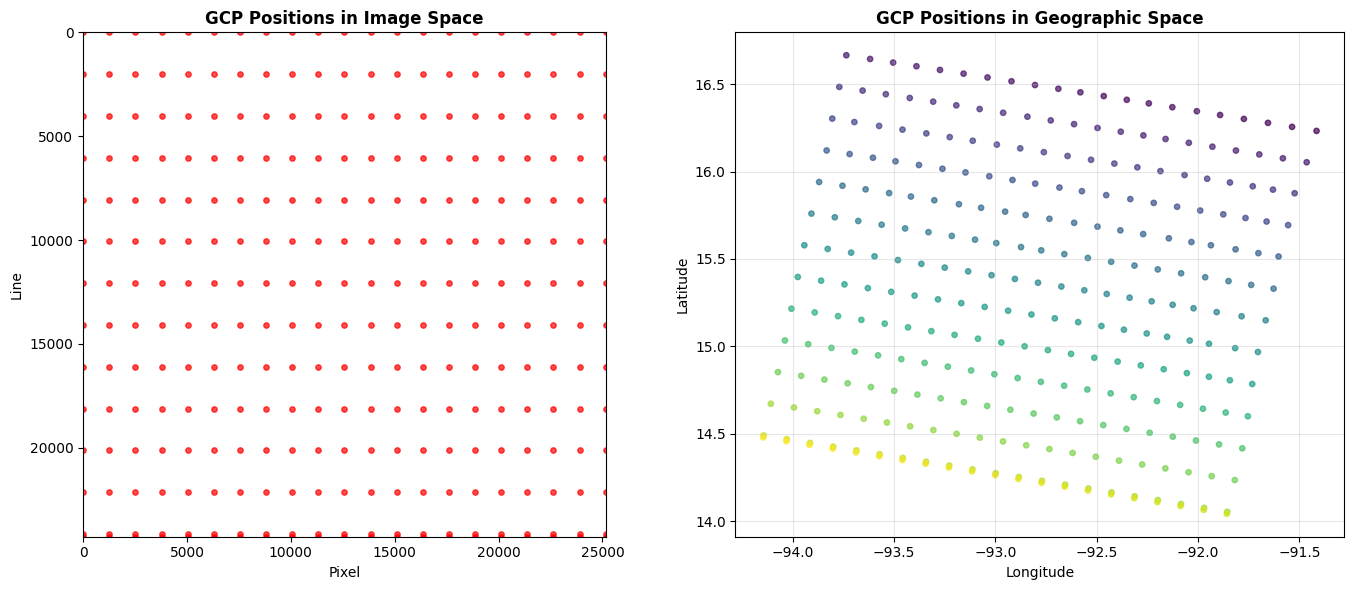
GCP grid: 21 columns x 14 rows = 294 points
Sampling: ~1 GCP every 1197 pixels (range) x 1734 pixels (azimuth)
Pixel-to-Geographic Coordinate Transformation
With GCPs attached, GDAL can transform between pixel coordinates and geographic coordinates using a GCP-based transformer.
# Create a GCP-based transformer
transformer = gdal.Transformer(ds, None, ["METHOD=GCP_POLYNOMIAL", "MAX_GCP_ORDER=3"])

# Transform image corners to geographic coordinates
corners = [
    ("Top-Left", 0, 0),
    ("Top-Right", ds.RasterXSize, 0),
    ("Bottom-Left", 0, ds.RasterYSize),
    ("Bottom-Right", ds.RasterXSize, ds.RasterYSize),
    ("Center", ds.RasterXSize // 2, ds.RasterYSize // 2),
]

print("Pixel-to-Geographic Coordinate Transformation:")
print(f"{'Location':<15} {'Pixel':>8} {'Line':>8}   {'Longitude':>12} {'Latitude':>12}")
print("-" * 65)
for name, px, ln in corners:
    success, result = transformer.TransformPoint(False, px, ln)
    if success:
        print(f"{name:<15} {px:>8} {ln:>8}   {result[0]:>12.4f} {result[1]:>12.4f}")
    else:
        print(f"{name:<15} {px:>8} {ln:>8}   transform failed")
Pixel-to-Geographic Coordinate Transformation:
Location Pixel Line Longitude Latitude
-----------------------------------------------------------------
Top-Left 0 0 -91.4285 16.2352
Top-Right 25157 0 -93.7365 16.6657
Bottom-Left 0 24285 -91.8581 14.0421
Bottom-Right 25157 24285 -94.1489 14.4795
Center 12578 12142 -92.7930 15.3590
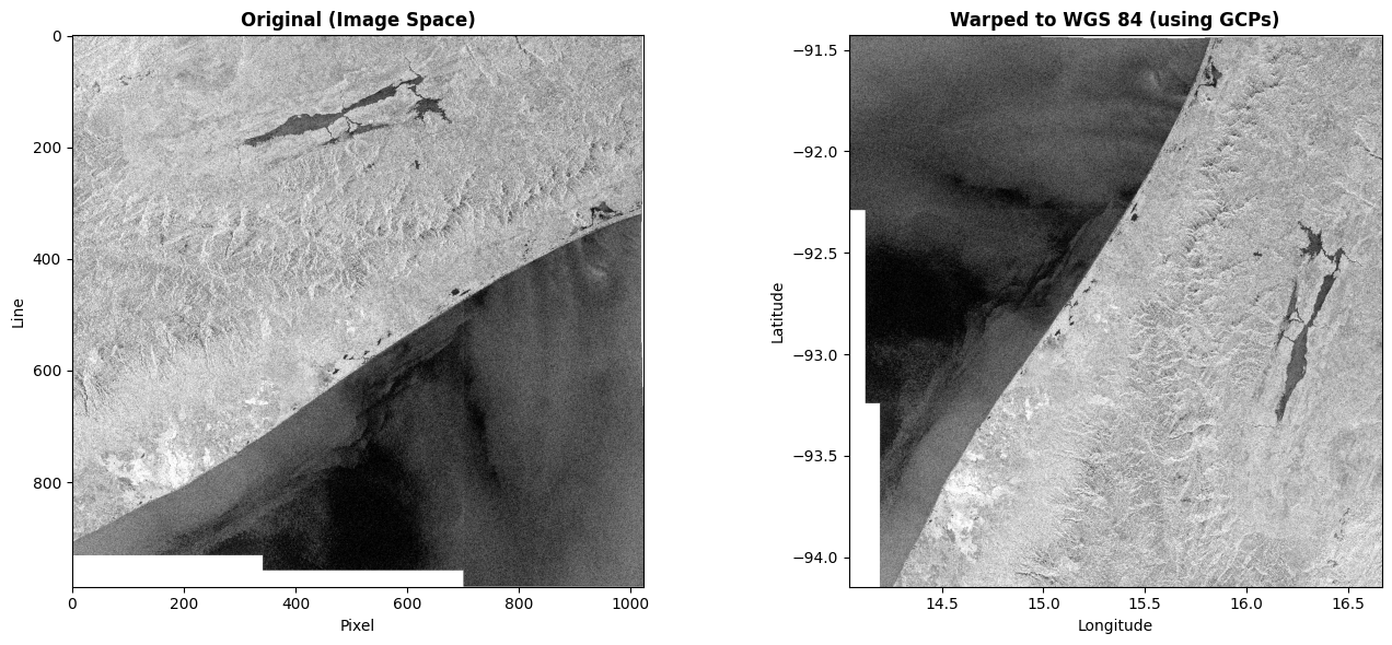
Warp to Geographic Projection
Using the GCPs, we can reproject the SAR data to a standard geographic projection (WGS 84). This is equivalent to what QGIS does when displaying GCP-based rasters.
# Warp a small subset to WGS 84 using GCPs
# We use a reduced resolution to keep it fast over /vsicurl/
warped = gdal.Warp(
    "",
    ds,
    format="MEM",
    dstSRS="EPSG:4326",
    width=1024,
    height=0,  # auto-compute from aspect ratio
    resampleAlg="near",
)

if warped:
    gt = warped.GetGeoTransform()
    print(f"Warped dataset: {warped.RasterXSize} x {warped.RasterYSize} pixels")
    print(
        f"GeoTransform:   origin=({gt[0]:.4f}, {gt[3]:.4f}), "
        f"pixel size=({gt[1]:.6f}, {gt[5]:.6f})"
    )
    print(f"Projection:     {warped.GetProjection()[:60]}...")

    try:
        data = warped.GetRasterBand(1).ReadAsArray()
        data_float = data.astype(np.float32)
        data_float[data_float == 0] = np.nan
        data_db = 10 * np.log10(data_float + 1)

        # Compute extent from geotransform
        extent = [
            gt[0],
            gt[0] + gt[1] * warped.RasterXSize,
            gt[3] + gt[5] * warped.RasterYSize,
            gt[3],
        ]

        fig, axes = plt.subplots(1, 2, figsize=(14, 6))

        # Original (pixel space)
        orig_sub = ds.GetRasterBand(1).ReadAsArray(
            buf_xsize=1024,
            buf_ysize=int(1024 * ds.RasterYSize / ds.RasterXSize),
        )
        orig_float = orig_sub.astype(np.float32)
        orig_float[orig_float == 0] = np.nan
        orig_db = 10 * np.log10(orig_float + 1)
        vmin, vmax = np.nanpercentile(orig_db, [2, 98])
        axes[0].imshow(orig_db, cmap="gray", vmin=vmin, vmax=vmax)
        axes[0].set_title("Original (Image Space)", fontweight="bold")
        axes[0].set_xlabel("Pixel")
        axes[0].set_ylabel("Line")

        # Warped (geographic space)
        vmin, vmax = np.nanpercentile(data_db, [2, 98])
        axes[1].imshow(data_db, cmap="gray", vmin=vmin, vmax=vmax, extent=extent)
        axes[1].set_title("Warped to WGS 84 (using GCPs)", fontweight="bold")
        axes[1].set_xlabel("Longitude")
        axes[1].set_ylabel("Latitude")

        plt.tight_layout()
        plt.show()
    except ImportError:
        print("ReadAsArray not available (NumPy version mismatch), skipping plot")

    warped = None
else:
    print("Warp failed")
Warped dataset: 1024 x 1060 pixels
GeoTransform: origin=(14.0422, -91.4289), pixel size=(0.002563, -0.002563)
Projection: GEOGCS["WGS 84",DATUM["WGS_1984",SPHEROID["WGS 84",6378137,2...
GCPs on SLC Burst Subdatasets
GCPs also work on SLC burst subdatasets. Let’s verify with a quick check.
SLC_URL = (
    "/vsicurl/https://objects.eodc.eu/e05ab01a9d56408d82ac32d69a5aae2a:"
    "notebook-data/tutorial_data/cpm_v262/"
    "S1C_IW_SLC__1SDV_20251016T165627_20251016T165654_004590_00913B_30C4.zarr"
)

ds_slc = gdal.OpenEx(
    f"EOPFZARR:'{SLC_URL}'", gdal.OF_RASTER, open_options=["BURST=IW1_VV_001"]
)

if ds_slc:
    slc_gcp_count = ds_slc.GetGCPCount()
    slc_srs = ds_slc.GetGCPSpatialRef()
    print("SLC Burst IW1_VV_001:")
    print(f"  Dimensions: {ds_slc.RasterXSize} x {ds_slc.RasterYSize}")
    print(f"  GCP Count:  {slc_gcp_count}")
    if slc_srs:
        print(f"  GCP SRS:    {slc_srs.GetName()}")

    if slc_gcp_count > 0:
        slc_gcps = ds_slc.GetGCPs()
        slc_lons = [g.GCPX for g in slc_gcps]
        slc_lats = [g.GCPY for g in slc_gcps]
        print(
            f"  Extent:     lon [{min(slc_lons):.4f}, {max(slc_lons):.4f}]"
            f"  lat [{min(slc_lats):.4f}, {max(slc_lats):.4f}]"
        )

    ds_slc = None
else:
    print("Failed to open SLC burst")
SLC Burst IW1_VV_001:
Dimensions: 23261 x 1501
GCP Count: 210
GCP SRS: WGS 84
Extent: lon [12.9673, 14.4821] lat [40.0726, 41.7453]
Command Line Usage
GCPs are visible via gdalinfo on a measurement subdataset (not the root dataset). You need to open a specific subdataset path to see the GCPs.
# Print the actual subdataset path used in this notebook
subds_path = vv_path.split("'")[1] if "'" in vv_path else vv_path

print("Step 1: List subdatasets\n")
print(f"  gdalinfo \"EOPFZARR:'{GRD_URL}'\" -oo GRD_MULTIBAND=NO\n")
print("Step 2: Open a measurement subdataset to see GCPs\n")
print(f"  gdalinfo '{subds_path}'\n")
print("The output will include:")
print('  GCP Projection = GEOGCS["WGS 84", ...]')
print("  GCP[  0]: Id=GCP_1, Info=")
print("            (0.5,0.5) -> (-91.4153, 16.2326, 574.99)")
print("  GCP[  1]: Id=GCP_2, Info=")
print("            (1258.5,0.5) -> (-91.5360, 16.2558, 904.98)")
print("  ...")
Step 1: List subdatasets
gdalinfo "EOPFZARR:'/vsicurl/https://objects.eodc.eu/e05ab01a9d56408d82ac32d69a5aae2a:notebook-data/tutorial_data/cpm_v264/S1C_IW_GRDH_1SDV_20260205T120122_20260205T120158_006220_00C7E4_5D6E.zarr'" -oo GRD_MULTIBAND=NO
Step 2: Open a measurement subdataset to see GCPs
gdalinfo 'EOPFZARR:"/vsicurl/https://objects.eodc.eu/e05ab01a9d56408d82ac32d69a5aae2a:notebook-data/tutorial_data/cpm_v264/S1C_IW_GRDH_1SDV_20260205T120122_20260205T120158_006220_00C7E4_5D6E.zarr":/S01SIWGRD_20260205T120122_0036_C036_5D6E_00C7E4_VV/measurements/grd'
The output will include:
GCP Projection = GEOGCS["WGS 84", ...]
GCP[ 0]: Id=GCP_1, Info=
(0.5,0.5) -> (-91.4153, 16.2326, 574.99)
GCP[ 1]: Id=GCP_2, Info=
(1258.5,0.5) -> (-91.5360, 16.2558, 904.98)
...
Summary
GCP Geolocation Features
| Feature | Description |
|---|---|
| Automatic Extraction | GCPs read from conditions/gcp/ arrays (pixel, line, latitude, longitude, height) |
| GCP SRS | WGS 84 (EPSG:4326) with traditional GIS axis ordering (lon, lat) |
| GRD Coverage | ~294 GCPs (14 x 21 sparse grid) per subdataset |
| SLC Coverage | ~210 GCPs (10 x 21 sparse grid) per burst |
| GDAL API | GetGCPCount(), GetGCPs(), GetGCPSpatialRef() |
| Reprojection | gdal.Warp() uses GCPs automatically for coordinate transformation |
How It Works
When a measurement subdataset is opened, the driver navigates up to the product root
It opens the five GCP arrays:
conditions/gcp/{pixel, line, latitude, longitude, height}The 1D
pixel/linearrays and 2Dlatitude/longitude/heightarrays are cross-referenced to build GDAL GCP structsGCPs are lazily loaded on first access to
GetGCPCount(),GetGCPs(), orGetGCPSpatialRef()
Usage
# Open a GRD subdataset - GCPs are automatically available
ds = gdal.Open(subdataset_path)
print(ds.GetGCPCount())         # e.g. 294
print(ds.GetGCPSpatialRef())    # WGS 84

# Reproject using GCPs
warped = gdal.Warp('output.tif', ds, dstSRS='EPSG:4326')

# Or use BURST for SLC
ds = gdal.OpenEx("EOPFZARR:'/vsicurl/...SLC...zarr'",
                 open_options=["BURST=IW1_VV_001"])
print(ds.GetGCPCount())         # e.g. 210
Cleanup
ds = None
print("All datasets closed")
All datasets closed