Computing Leaf Area Index with Sentinel-2 in EOPF Zarr format

Table of Contents¶

Run this notebook interactively with all dependencies pre-installed

Introduction¶

This notebook focuses on retrieving Leaf Area Index (LAI) from Sentinel-2 data using the Simplified Level 2 Prototype Processor (SL2P) framework [Weiss & Baret 2016] as implemented by Djamai et al., 2024.

LAI is a key biophysical variable for describing vegetation canopy structure and is defined “total leaf area per unit of ground area" [Watson, 1947]. In practice, LAI is widely used to monitor vegetation productivity, evapotranspiration, and drought through vegetation status and land–atmosphere interactions from remote sensing data.

SL2P is a physics-informed hybrid retrieval model. It is useful because it provides an operational way to estimate vegetation biophysical variables such as LAI from Sentinel-2 reflectance data. It combines simulations derived from the radiative transfer model PROSAIL [Jacquemoud et al., 2009] with deep learning based retrievals, making it suitable for large-scale, repeatable processing of satellite imagery.

This notebook is therefore useful both for understanding the SL2P workflow and for building a reproducible Python-based implementation for LAI retrieval.

Dj amai N., Fernandes, R.A. Sun. L., Canisius, F. and Hong. G, 2024. Python version of Simplified Level 2 Prototype Processor for Retrieving Canopy Biophysical Variables from Sentinel 2 Multispectral Instrument Data, Open File

Jacquemoud, S., Verhoef, W., Baret, F., Bacour, C., Zarco-Tejada, P. J., Asner, G. P., François, C., & Ustin, S. L. (2009). “PROSPECT+SAIL models: A review of use for vegetation characterization.” Remote Sensing of Environment, 113, S56–S66

Weiss, M., & Baret, F. (2016). S2ToolBox Level 2 Products: LAI, FAPAR, FCOVER (Version 1.1). Institut National de la Recherche Agronomique (INRA), Avignon, France.

Watson, D. J. (1947). Comparative physiological studies on the growth of field crops: I. Variation in net assimilation rate and leaf area between species and varieties, and within and between years. Annals of Botany, 11(41), 41–76

Setup¶

import os
import re
import sys
import time
import gc
import io
import warnings
import math
import xarray as xr
import xarray_eopf
from datetime import datetime
import matplotlib.pyplot as plt
import matplotlib.colors as colors
import numpy as np
import pandas as pd
import pystac_client
import geopandas as gpd
from contextlib import redirect_stdout
from pyproj import Transformer
from pathlib import Path
from joblib import Parallel, delayed
from typing import Tuple
import rasterio

sys.path.insert(0, os.path.join(os.getcwd(), "sl2p", "tools"))
sys.path.insert(0, os.path.join(os.getcwd(), "sl2p"))

from tools import SL2P, dictionariesSL2P
from tools.xarray_utils import varmap_to_dataset
from tools.xarray_utils import (
    ensure_angle_cosines,
    clip_cube_to_aoi,
    infer_profile,
)
from tools.xarray_utils import build_sl2p_input

## Ignore RuntimeWarning for data cast
warnings.filterwarnings("ignore", category=RuntimeWarning)

STAC Search¶

Define AOI and convert to raster CRS (area above Bolzano, South Tyrol, tile T32TPS)

spatial_extent = {
    "west": 11.317977240260499,
    "east": 11.3657883455519,
    "south": 46.483131171916064,
    "north": 46.50351101219372,
}

bbox_4326 = [
    spatial_extent["west"],
    spatial_extent["south"],
    spatial_extent["east"],
    spatial_extent["north"],
]

# Connect to the STAC catalog
catalog = pystac_client.Client.open("https://stac.core.eopf.eodc.eu")

# Search for Sentinel-2 L2A items within a specific bounding box and date range
search = catalog.search(
    collections=["sentinel-2-l2a"],
    bbox=bbox_4326,
    datetime="2023-04-30/2023-10-31",
)

# Retrieve the list of matching items
items = list(search.items())
items = [
    it
    for it in items
    # Filter only for cpm_v260 products, which are the ones we are interested in
    if any("cpm_v260" in asset.href.lower() for asset in it.assets.values())
]
hrefs = [item.assets["product"].href for item in items]

if not hrefs:
    raise RuntimeError(
        "No Sentinel-2 products matching the query in the STAC catalogue"
    )

SL2P biophysical variable retrieval¶

Preprocess input Sentinel-2 Zarr cubes and run SL2P on them .

Expected inputs:

10 m grid
Bands: B03,B04,B05,B06,B07,B8A,B11,B12 (SCL optional)
Angular features already as cosines: cosSZA, cosVZA, cosRAA

Parameters¶

In the original SL2P version, we could derive different types of variables (LAI, fAPAR, fCover, CCC, CWC, Albedo), from different types of input images (Sentinel-2, Landsat8/9, Harmonized Landsat-Sentinel), using two different algorithms (SL2P, SL2P-CCRS).

For the scope of this notebook, the possibilities have been reduced to the only case study of LAI from the SL2P algorithm using Sentinel-2 multispectral inputs

Furthemore, we can select whether the input data are already prescaled (PRESCALED_INPUT). Zarr cubes are already scaled to surface reflectance (0-1), so we skip SL2P pre-scaling.

We can choose to clip the input tile to an Area of Interest (AOI), and in this case we choose to clip the tile over some field polygons

variableName = "LAI"
imageCollectionName = "S2_10m"
method = "SL2P"

PRESCALED_INPUT = True

# (Opt.) Clipping to AOI - requires AOI shapefile. Reduces processing time and output file size.
clipping = True
AOI_path = "./geojson/renon_fields.geojson"

if clipping and not os.path.exists(AOI_path):
    raise FileNotFoundError(f"AOI shapefile not found: {AOI_path}")
if clipping:
    aoi = gpd.read_file(AOI_path)
    if aoi.empty:
        raise ValueError(f"AOI file contains no features: {AOI_path}")
    aoi = aoi.iloc[[0]]

out_dir = "./tmp/"

if clipping:
    out_dir = os.path.join(out_dir)
os.makedirs(out_dir, exist_ok=True)

Validation and options¶

This cells checks whether the conditions to create the neural network are met. If yes, it proceeds to extract the network options.

if variableName not in dictionariesSL2P.make_net_options():
    raise ValueError(f"Unsupported variable {variableName}")

net_options = dictionariesSL2P.make_net_options()[variableName][imageCollectionName]
required_inputs = net_options["inputBands"]
print(
    f"The required input layers for the SL2P {variableName} at 10 meters are: {required_inputs}"
)

The required input layers for the SL2P LAI at 10 meters are: ['cosVZA', 'cosSZA', 'cosRAA', 'B03', 'B04', 'B05', 'B06', 'B07', 'B8A', 'B11', 'B12']

Data preprocessing¶

Read the data from the urls obtained from the STAC Items
Combine the Sentinel-2 bands with the sun angles
Clips to the area of interest extent (minimum bounding box around it)
Stores the clipped pre-processed cube in a Zarr (necessary for memory management)
Finally recombines all the Zarr products into an Xarray Dataset loaded in memory

def prepare_sl2p_LAI_10m(url, aoi):
    # Use xarray-eopf to create a 10 m data cube and keep only the bands
    # required by the SL2P workflow.
    ds = xr.open_dataset(
        url,
        engine="eopf-zarr",
        op_mode="analysis",
        interp_methods="nearest",
    ).astype(np.float32)
    keys = list(ds.data_vars)
    values = [d.upper() for d in ds.data_vars]
    ds = ds.rename_vars(dict(zip(keys, values)))
    ds = ds[["B03", "B04", "B05", "B06", "B07", "B8A", "B11", "B12", "SCL"]]

    # Open the product as a DataTree to retrieve the sun and viewing angles,
    # then combine the interpolated angular cosines with the data cube.
    dt = xr.open_datatree(url, engine="zarr")
    product_datetime = dt.attrs["stac_discovery"]["properties"]["datetime"]
    SZA = (
        dt["conditions/geometry/sun_angles"]
        .sel(angle="zenith")
        .drop_vars("angle")
        .astype(np.float32)
    )
    SAA = (
        dt["conditions/geometry/sun_angles"]
        .sel(angle="azimuth")
        .drop_vars("angle")
        .astype(np.float32)
    )
    VZA_VAA = (
        dt["conditions/geometry/viewing_incidence_angles"]
        .loc[dict(band="b08")]
        .drop_vars("band")
        .mean(dim="detector")
        .astype(np.float32)
    )
    VZA = VZA_VAA.sel(angle="zenith").drop_vars("angle")
    VAA = VZA_VAA.sel(angle="azimuth").drop_vars("angle")
    RAA = np.absolute(SAA - VAA)

    ds["cosSZA"] = np.cos(np.deg2rad(SZA)).interp_like(ds)
    ds["cosVZA"] = np.cos(np.deg2rad(VZA)).interp_like(ds)
    ds["cosRAA"] = np.cos(np.deg2rad(RAA)).interp_like(ds)
    ds = ds.assign_coords(time=product_datetime).expand_dims("time")
    ds_clip = ds.loc[
        dict(
            x=slice(aoi.bounds.minx.item(), aoi.bounds.maxx.item()),
            y=slice(aoi.bounds.maxy.item(), aoi.bounds.miny.item()),
        )
    ]
    ds_clip.to_zarr(f"{out_dir}s2_preproc_{product_datetime}.zarr")
    del ds, ds_clip
    gc.collect()
    return

Run the data pre-processing in parallel using 3 cores. Max number on EOPF JupyterLab, otherwise the memory will be filled and the kernel will crash.

%%time
_ = Parallel(n_jobs=3)(delayed(prepare_sl2p_LAI_10m)(url, aoi) for url in hrefs)

CPU times: user 593 ms, sys: 277 ms, total: 870 ms
Wall time: 3min 31s

Open the multiple Zarr products as a single Xarray object:

ds_time_series = xr.open_mfdataset(
    [p for p in Path(out_dir).glob("*.zarr")],
    engine="zarr",
    chunks={},
    concat_dim="time",
    combine="nested",
    decode_cf=False,
    mask_and_scale=False,
).drop_vars("spatial_ref")
ds_time_series

Collect and summarize zonal statistics for a single polygon geometry on the SL2P LAI output. It applies the same quality masks as SL2P to ensure only valid pixels are included in the stats.

def summarize_single_polygon_lai(varmap_ds, variable_name, geometry, profile):
    lai = np.asarray(varmap_ds[variable_name].values, dtype=np.float32)
    valid = np.isfinite(lai)
    valid &= np.asarray(varmap_ds["sl2p_inputFlag"].values) == 0
    valid &= np.asarray(varmap_ds["sl2p_outputFlag"].values) == 0
    values = lai[
        rasterio.features.geometry_mask(
            [geometry],
            out_shape=lai.shape,
            transform=profile["transform"],
            invert=True,
            all_touched=True,
        )
        & valid
    ]
    return {
        "mean_lai": float(values.mean()) if values.size else np.nan,
        "median_lai": float(np.median(values)) if values.size else np.nan,
        "std_lai": float(values.std()) if values.size else np.nan,
        "n_valid_pixels": int(values.size),
    }

This function computes zonal statistics for all polygons in a GeoDataFrame on the SL2P LAI output and returns a GeoDataFrame ready for mapping.

def summarize_lai_by_polygons(varmap_ds, variable_name, polygons_gdf, profile):
    lai = np.asarray(varmap_ds[variable_name].values, dtype=np.float32)
    valid = np.isfinite(lai)
    valid &= np.asarray(varmap_ds["sl2p_inputFlag"].values) == 0
    valid &= np.asarray(varmap_ds["sl2p_outputFlag"].values) == 0

    polygons_projected = polygons_gdf.to_crs(profile["crs"]).copy()
    rows = []
    for _, row in polygons_projected.iterrows():
        mask = rasterio.features.geometry_mask(
            [row.geometry],
            out_shape=lai.shape,
            transform=profile["transform"],
            invert=True,
            all_touched=True,
        )
        values = lai[mask & valid]
        record = row.drop(labels="geometry").to_dict()
        record.update(
            {
                "geometry": row.geometry,
                "mean_lai": float(values.mean()) if values.size else np.nan,
                "median_lai": float(np.median(values)) if values.size else np.nan,
                "std_lai": float(values.std()) if values.size else np.nan,
                "n_valid_pixels": int(values.size),
            }
        )
        rows.append(record)

    return gpd.GeoDataFrame(rows, geometry="geometry", crs=polygons_projected.crs)

Main SL2P Algorithm¶

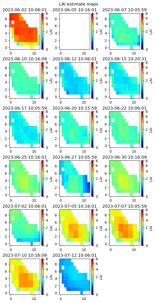
This cell iterates over the time series dataset, preparing inputs and then running the SL2P model to retrieve LAI for each timestep of the temporal window.

For each date, it optionally clips the data to the AOI, computes zonal statistics over the selected geometry, and stores the results in a time-ordered dataframe.

For the purposes of this specific notebook, it also shows the classified polygons for a brief temporal window from June to July 2023

from tqdm import tqdm

lai_stats_rows = []
stats_geometry = None
stats_geometry_crs = None

plot_start = pd.Timestamp("2023-06-01")
plot_end = pd.Timestamp("2023-07-15")

maps_to_plot = []

time_values = sorted(ds_time_series.time.values)

for idx, t in enumerate(tqdm(time_values, desc="Processing time steps"), start=1):
    start = time.time()
    time_value = pd.to_datetime(t.item(), utc=True).tz_localize(None)
    time_label = time_value.strftime("%Y-%m-%d %H:%M:%S")
    ds = ds_time_series.loc[dict(time=t)]

    source_ds = ds
    ds = ensure_angle_cosines(ds)

    ref_band = next((b for b in required_inputs if b in ds), None)
    if ref_band is None:
        raise ValueError(
            f"No required input bands found in dataset. Needed one of: {required_inputs}"
        )

    if clipping:
        ds, profile = clip_cube_to_aoi(ds, ref_band, AOI_path, required_inputs)
    else:
        profile = infer_profile(ds, ref_band, required_inputs)

    ############################
    # Build SL2P input and run the SL2P model
    sl2p_inp, dims = build_sl2p_input(ds, net_options, PRESCALED_INPUT)

    with warnings.catch_warnings(), redirect_stdout(io.StringIO()):
        warnings.filterwarnings(
            "ignore",
            message="invalid value encountered in cast",
            category=RuntimeWarning,
        )
        varmap = SL2P.SL2P(sl2p_inp, variableName, imageCollectionName, method)

    varmap_ds = varmap_to_dataset(varmap, template=ds, profile=profile)

    ############################
    # Store only selected dates for plotting later
    if plot_start <= time_value <= plot_end:
        valid_estimate = varmap_ds[variableName].where(
            varmap_ds["sl2p_outputFlag"] == 0
        )

        maps_to_plot.append({"time_label": time_label, "data": valid_estimate.copy()})
    ############################

    # Here we check if the geometry for zonal stats is in the same CRS as the SL2P output.
    # If not, we reproject it on the fly.
    if stats_geometry_crs != str(profile["crs"]):
        stats_geometry = aoi.to_crs(profile["crs"]).geometry.iloc[0]
        stats_geometry_crs = str(profile["crs"])

    # Compute zonal stats for the current time step and append to results list
    lai_stats_rows.append(
        {
            "time": time_value,
            **summarize_single_polygon_lai(
                varmap_ds, variableName, stats_geometry, profile
            ),
        }
    )

    if hasattr(source_ds, "close"):
        source_ds.close()

    del ds, sl2p_inp, varmap, varmap_ds
    gc.collect()

#############################
# Plot the LAI maps for the selected dates. Only valid estimates are shown (outputFlag == 0).
if maps_to_plot:
    ncols = 3
    nrows = math.ceil(len(maps_to_plot) / ncols)

    fig, axes = plt.subplots(
        nrows, ncols, figsize=(6, 2 * nrows), constrained_layout=True
    )
    axes = np.ravel(axes)

    norm = colors.PowerNorm(gamma=0.5, vmin=0, vmax=8)

    for ax, item in zip(axes, maps_to_plot):
        item["data"].plot(
            ax=ax, cmap="jet", norm=norm, cbar_kwargs={"label": variableName}
        )
        ax.set(title=item["time_label"], xlabel="", ylabel="")

    for ax in axes[len(maps_to_plot) :]:
        ax.axis("off")

    plt.suptitle(f"{variableName} estimate maps")
    plt.show()
#############################

lai_stats_df = pd.DataFrame(lai_stats_rows).sort_values("time").reset_index(drop=True)

print("Processing complete")
lai_stats_df

Processing time steps: 100%|██████████| 74/74 [00:13<00:00,  5.47it/s]

Processing complete

LAI time series¶

Visualize the time-series of the zonal statistics collected over the plot. For each valid data point we will visualize the mean, the median, and the standard deviation.

if lai_stats_df.empty:
    raise ValueError("No zonal statistics available to plot.")

plot_df = lai_stats_df.sort_values("time")
lower = plot_df["mean_lai"] - plot_df["std_lai"]
upper = plot_df["mean_lai"] + plot_df["std_lai"]

fig, ax = plt.subplots(figsize=(12, 5))
ax.plot(plot_df["time"], plot_df["mean_lai"], marker="o", label="Mean LAI")
ax.plot(plot_df["time"], plot_df["median_lai"], marker="s", label="Median LAI")
ax.fill_between(plot_df["time"], lower, upper, alpha=0.2, label="Mean ± std")
ax.set_title("LAI Time Series")
ax.set_xlabel("Date")
ax.set_ylabel("LAI")
ax.grid(True, alpha=0.3)
ax.legend()
ax.tick_params(axis="x", rotation=45)
plt.show()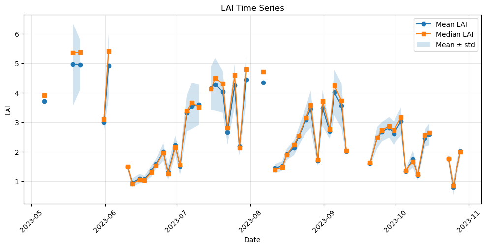

How can we interpret this graph showcasing the season evolution of canopy development and disturbance effects over a managed grassland field?

Early season (May–early June): LAI values are relatively high (~4–6), indicating a well-developed canopy. The variability suggests some spatial heterogeneity within the field, possibly linked to uneven growth or early management differences. There is not a lot of data, probably due to high cloud presence in early May.

Sharp drop (early June): The abrupt decrease to ~1–1.5 is characteristic of a mowing event, where biomass is removed. This marks a reset of the canopy.

Regrowth phase (June–July): LAI gradually increases, reflecting vegetation regrowth after mowing. The curve is relatively smooth, which is typical of continuous biomass accumulation.

Mid-season variability (July–August): You see fluctuations and occasional dips. These can be interpreted as: Secondary disturbances (e.g., mowing over multiple days → partial drops) Lodging effects, where flattened grass alters reflectance and leads to underestimated LAI Retrieval noise, especially when canopy structure is complex

Peak and second decline (August–September): Another growth peak (~3–4.5) is followed by a decline, again consistent with subsequent mowing cycles typical of managed grasslands.

Late season (September–October): Overall lower LAI with smaller amplitude cycles, indicating: Reduced regrowth capacity (seasonal effect) Continued management (smaller or partial cuts) Increased noise/outliers due to senescence, moisture changes, or residual biomass on the field.

Analysis of LAI Time Series¶

plot_df = lai_stats_df.sort_values("time").copy()
valid_df = plot_df.dropna(subset=["mean_lai"]).copy()

lower = plot_df["mean_lai"] - plot_df["std_lai"]
upper = plot_df["mean_lai"] + plot_df["std_lai"]
year = plot_df["time"].dt.year.mode().iat[0]

events = {
    "Mowing event": (["06-05", "08-09", "09-09", "10-07"], "red"),
    "Lodging date": (
        ["05-31", "06-27", "07-03", "07-22", "07-27", "08-30", "09-04"],
        "green",
    ),
}

prev_lai = valid_df["mean_lai"].shift(1)
next_lai = valid_df["mean_lai"].shift(-1)
neighbor_mean = (prev_lai + next_lai) / 2
absolute_drop_threshold = 0.75
relative_drop_threshold = 0.15
potential_outliers = valid_df[
    valid_df["mean_lai"].lt(prev_lai)
    & valid_df["mean_lai"].lt(next_lai)
    & neighbor_mean.sub(valid_df["mean_lai"]).ge(absolute_drop_threshold)
    & valid_df["mean_lai"].le(neighbor_mean * (1 - relative_drop_threshold))
]

fig, ax = plt.subplots(figsize=(12, 5))
ax.plot(
    plot_df["time"], plot_df["mean_lai"], marker="o", color="tab:blue", label="Mean LAI"
)
ax.plot(
    plot_df["time"],
    plot_df["median_lai"],
    marker="s",
    color="tab:orange",
    label="Median LAI",
)
ax.fill_between(
    plot_df["time"], lower, upper, alpha=0.2, color="tab:blue", label="Mean ± std"
)

for label, (dates, color) in events.items():
    for i, date in enumerate(pd.to_datetime([f"{year}-{d}" for d in dates])):
        ax.axvline(
            date,
            color=color,
            linestyle="--",
            linewidth=1.5,
            alpha=0.8,
            label=label if i == 0 else None,
        )

ax.set_title("LAI Time Series Analysis with Event Markers")
ax.set_xlabel("Date")
ax.set_ylabel("LAI")
ax.grid(True, alpha=0.3)
ax.legend()
ax.tick_params(axis="x", rotation=45)
plt.show()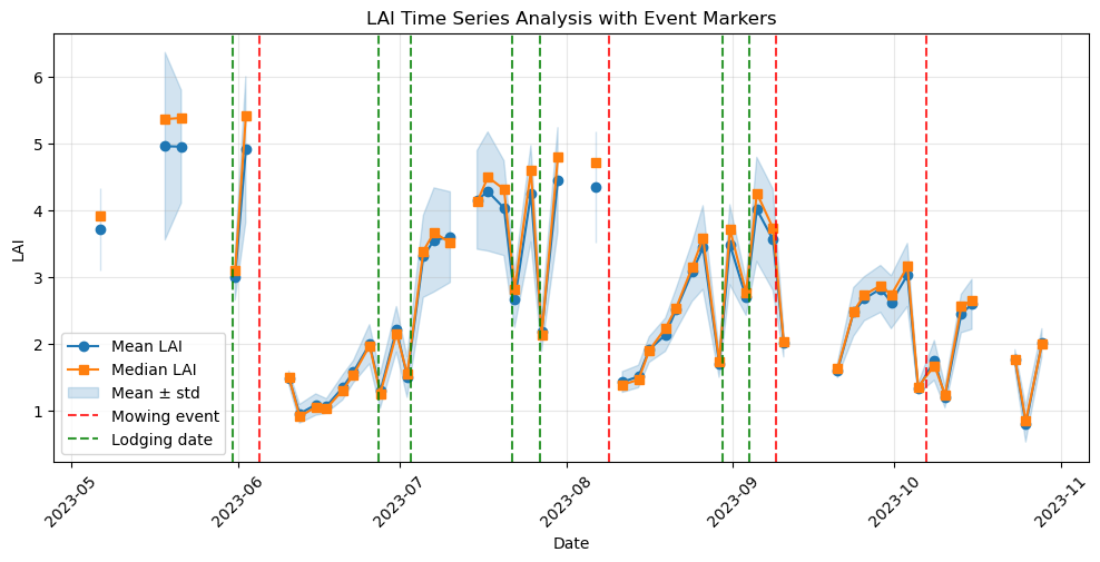

We could already spot some trends in the time series - but let’s add some context information.

The red dashed lines indicate possible occurrences of mowing events, that would explain the sudden drop and subsequent regrowth of LAI values. Following these dates, a decrease in LAI is expected in following observations, as biomass is removed. However, in some cases, grass is left on the field to dry after cutting, which can interfere with satellite retrieval and lead to inconsistencies in the estimated LAI values.

Additionally, mowing is not always performed uniformly across the field and may occur over multiple days. This can result in partial or gradual reductions in LAI rather than a sharp drop immediately after a single date.

The green dashed lines represent possible occurrences of lodging events. The observed patterns around these dates are consistent with lodging phenomena. Lodging is a phenomenon that occurs in grasslands when tall grass is bent over or is flattened due to strong weather events, such as rain storms or strong winds, or their own weight. This causes the canopy to lie more horizontally and alters light reflectance, affecting the estimation from satellite, leading to an apparent reduction in LAI in the satellite retrievals, even if the actual leaf area has not decreased.

Credits: Castelli, M., Mejia-Aguilar, A., Göhner, C., & Stendardi, L. (2025). Two years of in situ measurements of biophysical variables of mountain meadows in northeastern Italy [Data set]. Zenodo. Castelli et al. (2025)

References¶

Castelli, M., Mejia-Aguilar, A., Göhner, C., & Stendardi, L. (2025). Two years of in situ measurements of biophysical variables of mountain meadows in northeastern Italy. Zenodo. 10.5281/ZENODO.17984683