Building Sentinel-2 Data Cubes with xcube EOPF

Table of Contents¶

Introduction
Main Features of the xcube-eopf Data Store for Sentinel-2
Import modules
Access Sentinel-2 Level-2A ARDC
Access Sentinel-2 Level-1C ARDC
Conclusion

Run this notebook interactively with all dependencies pre-installed

Introduction¶

xcube-eopf is a Python package that extends xcube with a new data store called "eopf-zarr". This plugin enables the creation of analysis-ready data cubes (ARDC) from multiple Sentinel products published by the EOPF Sentinel Zarr Sample Service.

In this notebook, we demonstrate how to use the xcube EOPF data store to access multiple Sentinel-2 EOPF Zarr products and generate 3D analysis-ready data cubes (ARDC).

For a general introduction to the xcube EOPF Data Store, see the introduction notebook.

🐙 GitHub: EOPF Sample Service – xcube-eopf
❗ Issue Tracker: Submit or view issues
📘 Documentation: xarray-eopf Docs

Main Features of the xcube-eopf Data Store for Sentinel-2¶

Sentinel-2 provides multi-spectral imagery at different native spatial resolutions:

10 m: B02, B03, B04, B08
20 m: B05, B06, B07, B8A, B11, B12
60 m: B01, B09, B10

Sentinel-2 products are organized as STAC Items, each representing a single tile stored in its native UTM coordinate reference system (CRS).

Data Cube Generation Workflow¶

STAC Query: Relevant STAC Items (tiles) are retrieved via the STAC API based on the specified spatial and temporal extent (bbox and time_range).
Sorting: Items are ordered by acquisition time and tile ID.
Native Alignment: Within each UTM zone, tiles from the same acquisition day are aligned in their native CRS without reprojection. Overlapping pixels are resolved by selecting the first non-NaN value according to item order.
Cube Assembly: The cube generation strategy depends on the request, as summarized below:

Scenario	Native Resolution Preservation	Reprojected or Resampled Cube
Condition	Bounding box lies within a single UTM zone, the native CRS is requested, and the spatial resolution matches the native resolution.	Data spans multiple UTM zones, a different CRS is requested (e.g., EPSG:4326), or a custom spatial resolution is specified.
Processing	Only upsampling or downsampling is applied to align spectral bands with different resolutions. The cube is cropped to the requested bounding box, preserving original pixel values. The spatial extent may slightly adjust to the native grid.	A target grid is defined based on the bounding box, spatial resolution, and CRS. Data from each UTM zone is reprojected/resampled to this grid. Overlaps are resolved using the first non-NaN values.

Users can specify any spatial resolution and coordinate reference system (CRS) when calling open_data. Depending on the request, spectral bands may be resampled (upsampled or downsampled) and/or reprojected to match the target grid using xcube-resampling.

📚 More info: xcube-eopf Sentinel-2 Documentation

Import Modules¶

The xcube-eopf data store is provided as a plugin for xcube. Once installed, it registers automatically, allowing you to import xcube just like any other xcube data store:

import datetime
import matplotlib.colors as mcolors
import matplotlib.pyplot as plt
import numpy as np
from xcube.core.store import new_data_store
from xcube_resampling.utils import reproject_bbox

Access Sentinel-2 Level-2A ARDC¶

In this section, we demonstrate the available features and options for opening and generating spatio-temporal data cubes from multiple Sentinel-2 tiles.
To initialize an eopf-zarr data store, run the cell below:

store = new_data_store("eopf-zarr")

The data IDs point to STAC collections. In the following cell we can list the available data IDs.

store.list_data_ids()

['sentinel-2-l1c',
 'sentinel-2-l2a',
 'sentinel-3-olci-l1-efr',
 'sentinel-3-olci-l2-lfr',
 'sentinel-3-slstr-l1-rbt',
 'sentinel-3-slstr-l2-lst']

Below, you can explore the parameters of the open_data() method for each supported data product. The following cell generates a JSON schema listing all available opening parameters for Sentinel-2 Level-2A products.

store.get_open_data_params_schema(data_id="sentinel-2-l2a")

Spatio-Temporal Selection and Reprojection¶

We now generate a data cube from the Sentinel-2 L2A product by setting data_id to "sentinel-2-l2a".
The bounding box is defined to cover Mount Etna in Sicily, and the time range is set to the last 10 days.
We begin by creating the data cube in its native UTM projection to avoid any reprojection or sub-pixel resampling.

time_range = [str(datetime.date.today() - datetime.timedelta(days=10)), None]
bbox = [14.8, 37.45, 15.3, 37.85]
crs_utm = "EPSG:32633"
bbox_utm = reproject_bbox(bbox, "EPSG:4326", crs_utm)

%%time
ds = store.open_data(
    data_id="sentinel-2-l2a",
    bbox=bbox_utm,
    time_range=time_range,
    spatial_res=20,
    crs=crs_utm,
    variables=["b02", "b03", "b04", "scl"],
)
ds

CPU times: user 2.01 s, sys: 101 ms, total: 2.11 s
Wall time: 21.3 s

Note that the 3D datacube generation is fully lazy. Actual data download and processing (e.g., mosaicking, stacking) are performed on demand and are only triggered when the data is written or visualized.

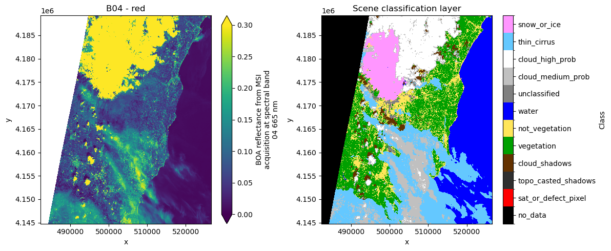
As an example, the next cell plots a single timestamp of the red band and the Scene Classification Layer (SCL). The plot uses the color map information provided in the attributes of the SCL data array.

fig, ax = plt.subplots(1, 2, figsize=(12, 5))

ds.b04.isel(time=-2).plot(ax=ax[0], vmin=0.0, vmax=0.3)
ax[0].set_title("B04 - red")

cmap = mcolors.ListedColormap(ds.scl.attrs["flag_colors"].split(" "))
nb_colors = len(ds.scl.attrs["flag_values"])
norm = mcolors.BoundaryNorm(
    boundaries=np.arange(nb_colors + 1) - 0.5, ncolors=nb_colors
)
im = ds.scl.isel(time=-2).plot.imshow(
    ax=ax[1], cmap=cmap, norm=norm, add_colorbar=False
)
cbar = fig.colorbar(im, ax=ax[1], ticks=ds.scl.attrs["flag_values"])
cbar.ax.set_yticklabels(ds.scl.attrs["flag_meanings"].split(" "))
cbar.set_label("Class")
ax[1].set_title("Scene classification layer")

plt.tight_layout()

/home/konstantin/micromamba/envs/xcube-eopf/lib/python3.13/site-packages/numpy/_core/numeric.py:475: RuntimeWarning: invalid value encountered in cast
  multiarray.copyto(res, fill_value, casting='unsafe')
/home/konstantin/micromamba/envs/xcube-eopf/lib/python3.13/site-packages/dask/array/chunk.py:288: RuntimeWarning: invalid value encountered in cast
  return x.astype(astype_dtype, **kwargs)

The user can also set crs="native" which allows specifying the bounding box in latitude/longitude, but returns the data in UTM. Note if the data request covers multiple UTM zones, an error will be raised.

ds = store.open_data(
    data_id="sentinel-2-l2a",
    bbox=bbox,
    time_range=time_range,
    spatial_res=10,
    crs="native",
    variables=["b02", "b03", "b04", "scl"],
)
ds

We can request the same data cube but in geographic projection (“EPSG:4326”) as well. The xcube EOPF data store can reproject the datacube to any projection requested by the user.

ds = store.open_data(
    data_id="sentinel-2-l2a",
    bbox=bbox,
    time_range=time_range,
    spatial_res=20 / 111320,  # meters converted to degrees (approx.)
    crs="EPSG:4326",
    variables=["b02", "b03", "b04", "scl"],
)
ds

ds.b04.isel(time=-2).plot(vmin=0, vmax=0.2)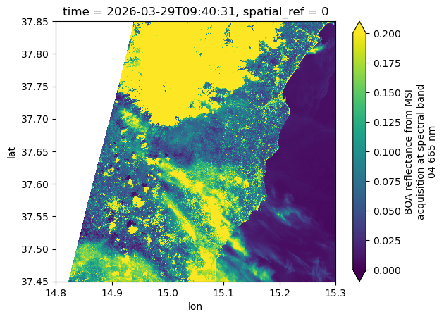

Support for Common Band Names¶

Support has been added for common band names from the STAC EO extension in Sentinel-2 analysis mode.

The variables parameter now accepts standard spectral names such as blue, green, red, nir, and others.

The next cell demonstrates an example where we filter spectral bands using these common names.

ds = store.open_data(
    data_id="sentinel-2-l2a",
    bbox=bbox,
    time_range=time_range,
    spatial_res=20 / 111320,  # meters converted to degrees (approx.)
    crs="EPSG:4326",
    variables=["blue", "green", "red", "scl"],
)
ds

Access Sentinel-2 Level-1C ARDC¶

In this section, we demonstrate how to open and generate spatio-temporal data cubes from multiple Sentinel-2 Level-1C tiles.

The Level-1C collection uses the same opening parameters as the Level-2A collection, as shown below.

store.get_open_data_params_schema(data_id="sentinel-2-l1c")

We set data_id to "sentinel-2-l1c" and leave variables unspecified, so all spectral bands are retrieved. We also do not set a crs, so the default "EPSG:4326" is used.

ds = store.open_data(
    data_id="sentinel-2-l1c",
    bbox=bbox,
    time_range=time_range,
    spatial_res=20 / 111320,  # meters converted to degrees (approx.)
)
ds

And we can plot a spectral band for a time stamp, which triggers loading the data for this slice.

ds.b04.isel(time=-2).plot(vmin=0, vmax=0.2)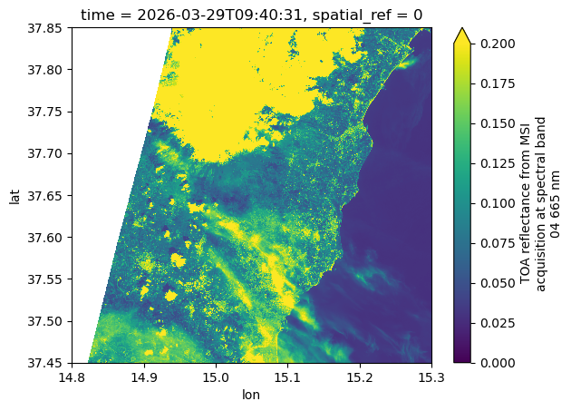

Conclusion¶

This notebook highlighted the main features of the xcube EOPF Data Store for Sentinel-2, which enables seamless access to multiple EOPF Zarr products as analysis-ready data cubes (ARDCs).

Key takeaways:

3D spatio-temporal data cubes can be generated from multiple EOPF Sentinel Zarr samples.
Supports access to both Sentinel-2 Level-2A and Level-1C collections.
Data cubes can be requested with any CRS, spatial extent, temporal range, and spatial resolution.
Setting crs="native" preserves the original UTM grid; an error is raised if the requested spatial extent spans multiple UTM zones.
Common spectral bands, as defined by the STAC EO extension, are supported for variable selection.