Building Sentinel-3 Data Cubes with xcube EOPF

Table of Contents¶

Introduction
Main Features of the xcube-eopf Data Store for Sentinel-2
Import modules
Access Sentinel-3 ARDC
Conclusion

Run this notebook interactively with all dependencies pre-installed

Introduction¶

xcube-eopf is a Python package that extends xcube with a new data store called "eopf-zarr". This plugin enables the creation of analysis-ready data cubes (ARDC) from multiple Sentinel products published by the EOPF Sentinel Zarr Sample Service.

In this notebook, we demonstrate how to use the xcube EOPF data store to access multiple Sentinel-3 EOPF Zarr products and generate 3D analysis-ready data cubes (ARDC).

For a general introduction to the xcube EOPF Data Store, see the introduction notebook.

🐙 GitHub: EOPF Sample Service – xcube-eopf
❗ Issue Tracker: Submit or view issues
📘 Documentation: xarray-eopf Docs

Main Features of the xcube-eopf Data Store for Sentinel-3¶

Sentinel-3 has two instruments on board:

🌊 OLCI — Ocean and Land Colour Instrument

Purpose: Primarily designed for ocean and land surface monitoring.
Spectral bands: 21 bands (400–1020 nm).
Spatial resolution: 300 m.
Swath width: ~1,270 km

🔥 SLSTR — Sea and Land Surface Temperature Radiometer

Purpose: Measures global sea and land surface temperatures with high accuracy.
Spectral bands: 9 bands (visible to thermal infrared, 0.55–12 μm).
Spatial resolution: 500 m (visible & shortwave infrared bands) and 1 km (thermal infrared bands).
Swath width: ~1,400 km

Sentinel-3 data products are distributed as STAC Items, where each item corresponds to a single tile. The datasets are provided in their native 2D irregular grid and typically require rectification for analysis-ready applications.

Data Cube Generation Workflow

The workflow for building 3D analysis-ready cubes from Sentinel-3 products involves the following steps:

Query tiles using the EOPF Zarr Sample Service STAC API for a given time range and spatial extent.
Group items by solar day and orbit direction (ascending and descending passes).
Rectify data from the native 2D irregular grid to a regular grid using xcube-resampling.
Mosaic adjacent tiles into seamless daily scenes.
Stack the daily mosaics along the temporal axis to form 3D data cubes for each variable (e.g., spectral bands).

Note: Rectification (irregular → regular grid) is computationally expensive and may slow down cube generation.

📚 More info: xcube-eopf Sentinel-3 Documentation

Import Modules¶

The xcube-eopf data store is provided as a plugin for xcube. Once installed, it registers automatically, allowing you to import xcube just like any other xcube data store:

import datetime
import matplotlib.pyplot as plt
from xcube.core.store import new_data_store
from xcube_resampling.utils import reproject_bbox

Access Sentinel-3 ARDC¶

In this section, we demonstrate the available features and options for opening and generating spatio-temporal data cubes from multiple Sentinel-3 products.
To initialize an eopf-zarr data store, run the cell below:

store = new_data_store("eopf-zarr")

The data IDs refer to STAC collections available via the STAC Browser. The following cell demonstrates how to list the available data IDs.

For Sentinel-3, the following STAC collections are currently accessible through xcube-eopf:

Data ID	Description
“sentinel-3-olci-l1-efr”	Level-1 full-resolution top-of-atmosphere radiances from OLCI
“sentinel-3-olci-l2-lfr”	Level-2 land and atmospheric geophysical parameters derived from OLCI
“sentinel-3-slstr-l1-rbt”	Level-1 radiances and brightness temperatures from SLSTR
“sentinel-3-slstr-l2-lst”	Level-2 land surface temperature products from SLSTR

store.list_data_ids()

['sentinel-2-l1c',
 'sentinel-2-l2a',
 'sentinel-3-olci-l1-efr',
 'sentinel-3-olci-l2-lfr',
 'sentinel-3-slstr-l1-rbt',
 'sentinel-3-slstr-l2-lst']

Access Sentinel-3 OLCI L1 EFR ARDC¶

Below, you can explore the parameters of the open_data() method for each supported data product. The following cell generates a JSON schema listing all available opening parameters for Sentinel-3 OLCI L1 EFR products.

store.get_open_data_params_schema(data_id="sentinel-3-olci-l1-efr")

Next, we generate a data cube by setting the data_id to "sentinel-3-olci-l1-efr". The spatial extent is defined using a bounding box over Southern Italy, while the temporal range is restricted to the last two days. The coordinate reference system (CRS) is set to WGS84 (EPSG:4326) by default.

bbox = [14.0, 37.0, 18.0, 41.0]
time_range = [str(datetime.date.today() - datetime.timedelta(days=2)), None]
resolution = 300  # meter
variables = ["oa02_radiance", "oa04_radiance", "oa06_radiance"]  # RGB bands

ds = store.open_data(
    data_id="sentinel-3-olci-l1-efr",
    bbox=bbox,
    time_range=time_range,
    spatial_res=resolution / 111320,  # conversion to degree approx.
    variables=variables,
)
ds

Note that the 3D datacube generation is fully lazy. Actual data download and processing (e.g., mosaicking, stacking) are performed on demand and are only triggered when the data is written or visualized.

As an example, the next cell plots a single timestamp of the red band (oa06_radiance).

ds.oa06_radiance.isel(time=0).plot(vmax=100)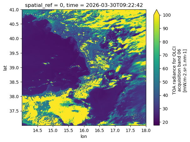

We can also request the same data cube in a different coordinate reference system (CRS), such as UTM. The xcube-eopf framework supports on-the-fly reprojection to any user-defined CRS.

Resampling behavior can be customized if needed. By default, bilinear interpolation is applied to floating-point data, while nearest-neighbor interpolation is used for integer data. For aggregation, float arrays use averaging, and integer arrays use a center-based approach. (see xcube-resampling docuementation)

If the requested spatial resolution is coarser than the native resolution, the data are first aggregated and then reprojected, with interpolation applied during the reprojection step.

crs_utm = "EPSG:32632"
bbox_utm = reproject_bbox(bbox, "EPSG:4326", crs_utm)

ds = store.open_data(
    data_id="sentinel-3-olci-l1-efr",
    bbox=bbox_utm,
    time_range=time_range,
    spatial_res=resolution,
    variables=variables,
    crs=crs_utm,
    interp_methods="nearest",
    agg_methods="center",
)
ds

ds.oa06_radiance.isel(time=0).plot(vmax=100)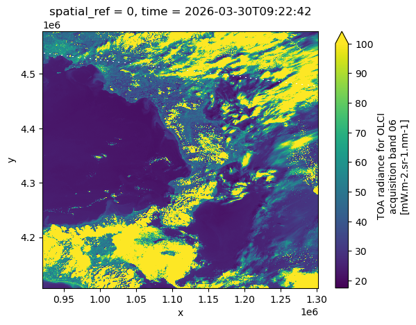

Access Sentinel-3 OLCI Level-2 LFR ARDC¶

We now want to generate a similar data cube from the Sentinel-3 OLCI Level-2 LFR product. We therefore assign data_id to "sentinel-3-olci-l2-lfr".

ds = store.open_data(
    data_id="sentinel-3-olci-l2-lfr",
    bbox=bbox,
    time_range=time_range,
    spatial_res=resolution / 111320,  # conversion to degree approx.
)
ds

ds.otci.isel(time=0).plot(robust=True)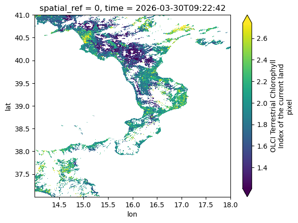

Access Sentinel-3 SLSTR Level-2 LST¶

Next, we want to generate a similar data cube from the Sentinel-3 SLSTR Level-2 LST product. We therefore assign data_id to "sentinel-3-slstr-l2-lst".

For SLSTR products, a terrain correction is applied during this process. This is necessary because the original geolocation is corrected only for Earth curvature, but not for terrain variability caused by topography. See the SLSTR product description for details.

ds = store.open_data(
    data_id="sentinel-3-slstr-l2-lst",
    bbox=bbox,
    time_range=time_range,
    spatial_res=resolution / 111320,  # conversion to degree approx.
)
ds

ds.lst.isel(time=0).plot(robust=True)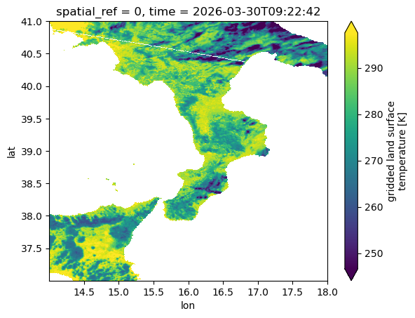

Access Sentinel-3 SLSTR Level-1B RBT¶

Lastly, we generate a similar data cube from the Sentinel-3 SLSTR Level-1B RBT product by setting data_id to "sentinel-3-slstr-l1-rbt".

The SLSTR instrument provides observations from two viewing geometries: nadir and oblique (forward view). These are designed to improve atmospheric correction and enable more accurate surface measurements.

Accordingly, many variables in the RBT product are available in pairs:

*_an → nadir view (e.g. s1_radiance_an)
*_ao → oblique view (e.g. s1_radiance_ao)

In the next example, we request both views for the S1 thermal channel.

ds = store.open_data(
    data_id="sentinel-3-slstr-l1-rbt",
    bbox=bbox,
    time_range=time_range,
    spatial_res=resolution / 111320,  # conversion to degree approx.
    variables=["s1_radiance_an", "s1_radiance_ao"],
)
ds

As an example, we plot the nadir and oblique views of the S1 thermal channel side by side.

fig, ax = plt.subplots(1, 2, figsize=(12, 5))
ds.s1_radiance_an.isel(time=0).plot(ax=ax[0], vmax=100)
ds.s1_radiance_ao.isel(time=0).plot(ax=ax[1], vmax=100)
plt.tight_layout()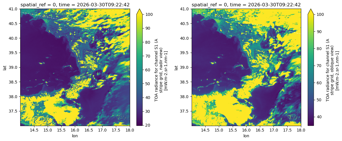

Conclusion¶

This notebook highlighted the main features of the xcube EOPF Data Store for Sentinel-3, which enables seamless access to multiple EOPF Zarr products as analysis-ready data cubes (ARDCs).

Key takeaways:

3D spatio-temporal data cubes can be generated from multiple EOPF Sentinel Zarr samples.
Supports access to Sentinel-3 OLCI L1 EFR, Sentinel-3 OLCI Level-2 LFR, Sentinel-3 SLSTR Level-2 LST, and Sentinel-3 SLSTR Level-1B RBT collections.
Data cubes can be requested with any CRS, spatial extent, temporal range, and spatial resolution.