Sentinel-1 SLC Zarr Product Exploration

Sentinel-1 SLC Zarr Product Exploration¶

Run this notebook interactively with all dependencies pre-installed

Table of Contents¶

Introduction
Import modules
File path definition
Open the product
Metadata Inspection
Overview of the product content
Examples of product usage
Amplitude and Intensity
Multi-Look
Calibration
Geocoding using GCPs
RGB Plot of two non coregistred burst

Introduction¶

This notebook demonstrates how to open, explore, process and visualize Sentinel-1 Interferometric Wide (IW) SLC products stored in EOPF Zarr format, including accessing, calibrating, geocoding, subsetting and plotting.

Import modules¶

import numpy as np
import xarray as xr
import matplotlib.pyplot as plt
import cartopy.crs as ccrs

xr.set_options(display_expand_attrs=False)

<xarray.core.options.set_options at 0x7f70ee2b2150>

Products Definition¶

SLC Product 1: S1A_IW_SLC__1SDV_20231119T170635_20231119T170702_051289_063021_178F
SLC Product 2: S1A_IW_SLC__1SDV_20231201T170634_20231201T170701_051464_06361B_A27C

Remote files URLs

remote_product_url_1 = "https://objects.eodc.eu:443/e05ab01a9d56408d82ac32d69a5aae2a:notebook-data/tutorial_data/cpm_v260/S1A_IW_SLC__1SDV_20231119T170635_20231119T170702_051289_063021_178F.zarr"
remote_product_url_2 = "https://objects.eodc.eu:443/e05ab01a9d56408d82ac32d69a5aae2a:notebook-data/tutorial_data/cpm_v260/S1A_IW_SLC__1SDV_20231201T170634_20231201T170701_051464_06361B_A27C.zarr"

Open the product¶

The SLC product can be opened as a DataTree using Xarray, where each group represents one burst:

dt = xr.open_datatree(remote_product_url_1, engine="zarr", chunks={})
dt

Metadata Inspection¶

When you work with Sentinel-1 data, you typically want to know the product location, the orbit direction and number, which are necessary information to consider if you would like to work with combination of products. We can find these in the product attributes.

Explore product geolocation¶

The Zarr product metadata contains information about the product geolocation we can explore in various ways. For instance, we can show the product footprint on an interactive map.

import geopandas as gpd

# Create a GeoDataFrame from the feature
gdf = gpd.GeoDataFrame.from_features(
    [
        {
            "type": "Feature",
            "geometry": dt.attrs["stac_discovery"][
                "geometry"
            ],  # Use the actual geometry, not the bbox
            "properties": dt.attrs["stac_discovery"][
                "properties"
            ],  # Include all properties
        }
    ],
    crs="EPSG:4326",  # Set the CRS explicitly
)
gdf.explore()

Get Orbit Information¶

In the properties field of the STAC metadata, we can find the required orbit values:

dt.attrs["stac_discovery"]["properties"]

{'constellation': 'sentinel-1',
 'created': '2023-11-19T17:54:50.000000Z',
 'datetime': '2023-11-19T17:06:48.793220Z',
 'end_datetime': '2023-11-19T17:07:02.279725Z',
 'eopf:datatake_id': '405537',
 'eopf:instrument_mode': 'IW',
 'instruments': 'sar',
 'platform': 'sentinel-1a',
 'processing:software': {'name': 'Sentinel-1 EOPF', 'version': '2.5.8'},
 'product:timeliness': 'PT3H',
 'product:timeliness_category': 'NRT-3h',
 'product:type': 'S01SIWSLC',
 'provider': [{'name': 'Copernicus Ground Segment', 'roles': ['processor']},
  {'name': 'ESA', 'roles': ['producer']}],
 'sar:frequency_band': 'C',
 'sar:instrument_mode': 'IW',
 'sar:polarizations': ['VV', 'VH'],
 'sat:absolute_orbit': 51289,
 'sat:anx_datetime': '2023-11-19T16:55:04.389887',
 'sat:orbit_state': 'ascending',
 'sat:platform_international_designator': '2014-016A',
 'sat:relative_orbit': 117,
 'start_datetime': '2023-11-19T17:06:35.306715Z'}

orbit_direction = dt.attrs["stac_discovery"]["properties"]["sat:orbit_state"]
orbit_number = dt.attrs["stac_discovery"]["properties"]["sat:relative_orbit"]

print("Orbit Direction: ", orbit_direction, "\nOrbit Number: ", orbit_number)

Orbit Direction:  ascending 
Orbit Number:  117

Overview of the product content¶

IW SLC products consist of three sub-swaths images per polarization channel, for a total of three (single polarizations) or six (dual polarization) images in an IW product. Each sub-swath image consists of a series of bursts, where each burst has been processed as a separate SLC image.

The bursts are the light blue rectangles in the figure below. The sub-swath (IW1) is composed by the bursts highlighted in red.

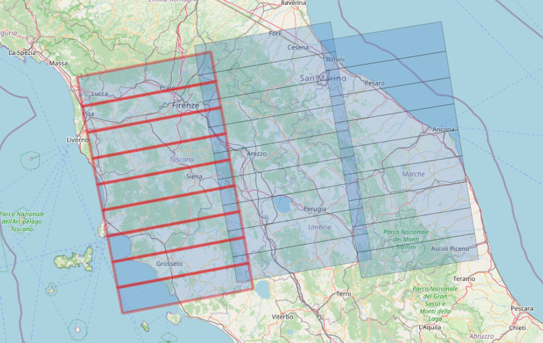
If you want to know more, please refer to: https://sentiwiki.copernicus.eu/web/s1-products

Sentinel-1 bursts in blue and sub-swath IW1 highlighted in red

Map data by OpenStreetMap

The EOPF Zarr SLC product contains one group for each burst. Each burst is identified by the following elements:

Polarization: typically VV or VH
Sub-swath: IW1, IW2 or IW3
Burst Id

How many burst does this product contain for each polarization?

We can count how many children of the DataTree contain the VH polarization. Each children correspond to a burst.

polarization = "VH"
bursts_VH = [x for x in dt.children if polarization in x]
print(
    f"The product contains {len(bursts_VH)} burst for the polarization {polarization}"
)

The product contains 27 burst for the polarization VH

Examples of product usage¶

SLC data extraction¶

The SLC (Single Look Complex) data is located in the measurements/slc group.

subswath = "IW1"
polarization = "VH"
burst_id = "249411"

burst_group = [
    x
    for x in dt.children
    if (polarization in x) and (subswath in x) and (burst_id in x)
][0]

burst_slc = dt[burst_group].measurements.slc.to_dataset()
burst_slc

Amplitude and Intensity¶

The amplitude of the complex signal can be computed as:

Amplitude = \sqrt {i^2 + q^2}

(1)

Where the intensity is the square of the amplitude:

Intensity = {i^2 + q^2}

(2)

We can compute them by extracting real and imaginary parts from the complex data:

burst_int = burst_slc.real**2 + burst_slc.imag**2
burst_amp = burst_int**0.5

Or also:

burst_amp = abs(burst_slc)
burst_int = burst_amp**2

Multi-Look¶

Multilook processing is an optional step and can be used to produce a product with nominal image pixel size.
Multiple looks may be generated by averaging over range and/or azimuth resolution cells improving radiometric resolution but degrading spatial resolution. As a result, the image will have less noise and approximate square pixel spacing after being converted from slant range to ground range.

For more info please visit: https://step.esa.int/docs/tutorials/S1TBX SAR Basics Tutorial.pdf

To perform multi-looking with Xarray, we use the coarsen method, together with .mean() to get the average over the window.

burst_amp_ml = burst_amp.coarsen(
    {"azimuth_time": 1, "slant_range_time": 5}, boundary="pad"
).mean()
burst_amp_ml

Calibration¶

We firstly need to extract the Calibration LUT (Lookup Table) values, located in the quality/calibration group.

calibration_lut = dt[burst_group].quality.calibration.to_dataset()
calibration_lut

Calibrate Data¶

You can get more information about this step at page 7 of this official ESA document.

calibration_matrix = calibration_lut.interp_like(burst_amp_ml)

# Calibrate Amplitude. Convert it to Intensity with power of 2.
sigma_nought = (burst_amp_ml / calibration_matrix["sigma_nought"]) ** 2

# Conversion to dB

sigma_nought_db = 10 * np.log10(sigma_nought)

/opt/conda/lib/python3.12/site-packages/dask/_task_spec.py:759: RuntimeWarning: divide by zero encountered in log10
  return self.func(*new_argspec)
/opt/conda/lib/python3.12/site-packages/dask/_task_spec.py:759: RuntimeWarning: divide by zero encountered in log10
  return self.func(*new_argspec)

Plot small subset¶

plt.figure(figsize=(5, 8))
sigma_nought_db.slc[:, 1350:1850].plot.imshow(vmin=-25, vmax=0)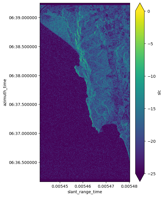

Geocoding using Ground Control Points (GCPs)¶

GCPs serve as anchor points that allow for precise alignment of satellite imagery with actual geographic locations.

Open GCP Data¶

gcp = dt[burst_group].conditions.gcp.to_dataset()
gcp

Interpolate and assign new geographic coordinates¶

gcp_iterpolated = gcp.interp_like(sigma_nought_db)
sigma_nought_db_gc = sigma_nought_db.slc.assign_coords(
    {"latitude": gcp_iterpolated.latitude, "longitude": gcp_iterpolated.longitude}
)

Plot geocoded subset¶

_, ax = plt.subplots(subplot_kw={"projection": ccrs.Miller()}, figsize=(12, 8))
gl = ax.gridlines(
    draw_labels=True, crs=ccrs.PlateCarree(), x_inline=False, y_inline=False
)
sigma_nought_db_gc[:, 1350:1850].plot(
    ax=ax, transform=ccrs.PlateCarree(), x="longitude", y="latitude", vmin=0, vmax=-20
)
ax.set_title("Geocoded sigma nought [dB]")
plt.show()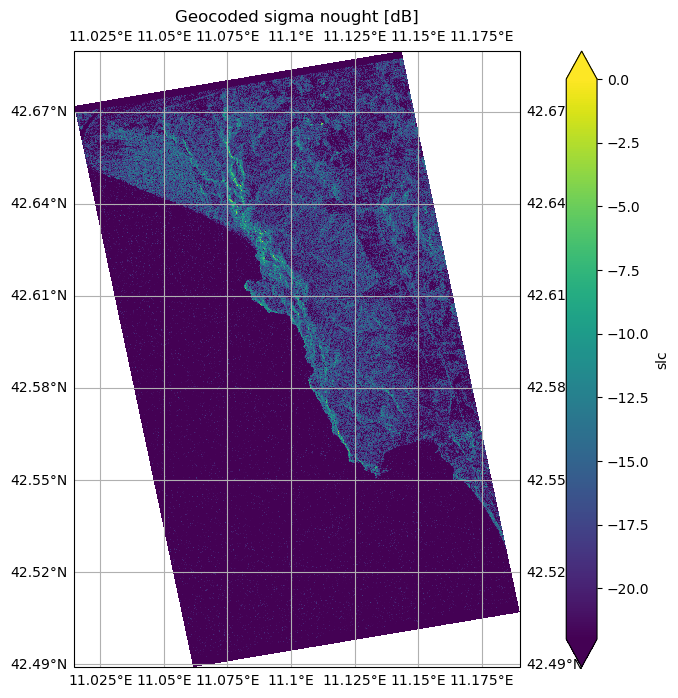

RGB Plot of two non coregistred burst¶

The RBG plot highlights the shift between the non co-registred bursts

subswath: IW1
polarization: VH
burst_id: 249411
burst acquisition date:
- 2023-12-01
- 2023-11-19

Open Data¶

dt2 = xr.open_datatree(remote_product_url_2, engine="zarr")
burst_group2 = [
    x
    for x in dt2.children
    if (polarization in x) and (subswath in x) and (burst_id in x)
][0]

burst_slc2 = dt2[burst_group2].measurements.slc.to_dataset()

burst_amp = burst_amp.drop_vars(["azimuth_time", "slant_range_time"])
burst_amp2 = abs(burst_slc2).drop_vars(["azimuth_time", "slant_range_time"])

Compose RGB¶

rgb = xr.concat([burst_amp, burst_amp, burst_amp2], dim="rgb")
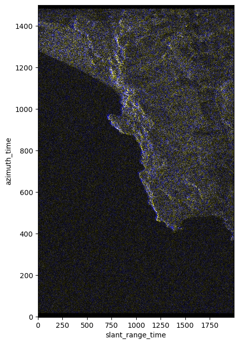
rgb = xr.where(rgb > 200, 200, rgb) / 200

Plot Subset¶

The following visualization will highlight the differences of the data acquired in the two different dates, which depend on the slight differences in the satellite orbit.
You will notice some blue areas, which highlight the areas with the highest values difference between the two dates.

To combine Sentinel-1 data samples from different dates as a time series, it’s necessary to co-register the images first for the best result, or work with the geocoded data.

plt.figure(figsize=(5, 8))
rgb.slc[:, :, 7000:9000].plot.imshow(rgb="rgb")
plt.show()

Welcome

Sentinel-1 GRD Zarr Product Exploration

Welcome

Sentinel-1 L2 OCN Zarr Product Exploration