Radar Vegetation Index

Radar Vegetation Index¶

🚀 Launch in JupyterHub

Run this notebook interactively with all dependencies pre-installed

Table of Contents¶

Preface
Introduction
Import Modules
Data Access
Spatial Slicing
Efficient Spatial Slicing
Calibration
Geocoding
Radar Vegetation Index
Time Series Analysis
Spatial Aggregation
Summary

Preface¶

The original notebooks used as a reference for this work are the following:

Copernicus Data Space Ecosystem example available here.
Sentinel Hub example, available here

The example has been adapted to use the data provided by the EOPF Sentinel Zarr Samples project instead of the openEO API or SentinelHub API.

Introduction¶

This notebook exmplains how to compute two different vegetation indexes using Sentinel-1 Ground Range Detected (GRD) data. They can be used to monitor the vegetation health condition or crop growth using SAR data.
We will use the Sentinel-1 GRD collection available within the EOPF Sentinel Zarr Samples STAC API, showing how to efficiently retrieve small Areas Of Interest (AOIs) from the data in SAR geometry.

Upgrade and install libraries:

pip install xarray --upgrade xvec

Requirement already satisfied: xarray in /home/mclaus@eurac.edu/micromamba/envs/eopf-zarr/lib/python3.11/site-packages (2025.1.1)
Collecting xarray
  Using cached xarray-2025.10.1-py3-none-any.whl.metadata (12 kB)
Collecting xvec
  Using cached xvec-0.5.1-py3-none-any.whl.metadata (3.2 kB)
Requirement already satisfied: numpy>=1.26 in /home/mclaus@eurac.edu/micromamba/envs/eopf-zarr/lib/python3.11/site-packages (from xarray) (1.26.4)
Requirement already satisfied: packaging>=24.1 in /home/mclaus@eurac.edu/micromamba/envs/eopf-zarr/lib/python3.11/site-packages (from xarray) (25.0)
Requirement already satisfied: pandas>=2.2 in /home/mclaus@eurac.edu/micromamba/envs/eopf-zarr/lib/python3.11/site-packages (from xarray) (2.3.3)
Requirement already satisfied: pyproj>=3.0.0 in /home/mclaus@eurac.edu/micromamba/envs/eopf-zarr/lib/python3.11/site-packages (from xvec) (3.7.2)
Requirement already satisfied: shapely>=2.0b1 in /home/mclaus@eurac.edu/micromamba/envs/eopf-zarr/lib/python3.11/site-packages (from xvec) (2.1.2)
Collecting cf_xarray>=0.9.2 (from xvec)
  Using cached cf_xarray-0.10.9-py3-none-any.whl.metadata (16 kB)
Collecting xproj>=0.2.0 (from xvec)
  Using cached xproj-0.2.1-py3-none-any.whl.metadata (3.0 kB)
Requirement already satisfied: python-dateutil>=2.8.2 in /home/mclaus@eurac.edu/micromamba/envs/eopf-zarr/lib/python3.11/site-packages (from pandas>=2.2->xarray) (2.9.0.post0)
Requirement already satisfied: pytz>=2020.1 in /home/mclaus@eurac.edu/micromamba/envs/eopf-zarr/lib/python3.11/site-packages (from pandas>=2.2->xarray) (2025.2)
Requirement already satisfied: tzdata>=2022.7 in /home/mclaus@eurac.edu/micromamba/envs/eopf-zarr/lib/python3.11/site-packages (from pandas>=2.2->xarray) (2025.2)
Requirement already satisfied: certifi in /home/mclaus@eurac.edu/micromamba/envs/eopf-zarr/lib/python3.11/site-packages (from pyproj>=3.0.0->xvec) (2025.11.12)
Requirement already satisfied: six>=1.5 in /home/mclaus@eurac.edu/micromamba/envs/eopf-zarr/lib/python3.11/site-packages (from python-dateutil>=2.8.2->pandas>=2.2->xarray) (1.17.0)
Using cached xarray-2025.10.1-py3-none-any.whl (1.4 MB)
Using cached xvec-0.5.1-py3-none-any.whl (784 kB)
Using cached cf_xarray-0.10.9-py3-none-any.whl (76 kB)
Using cached xproj-0.2.1-py3-none-any.whl (23 kB)
Installing collected packages: xarray, xproj, cf_xarray, xvec
  Attempting uninstall: xarray
    Found existing installation: xarray 2025.1.1
    Uninstalling xarray-2025.1.1:
      Successfully uninstalled xarray-2025.1.1
   ━━━━━━━━━━━━━━━━━━━━━━━━━━━━━━━━━━━━━━━━ 4/4 [xvec][32m1/4 [xproj]
ERROR: pip's dependency resolver does not currently take into account all the packages that are installed. This behaviour is the source of the following dependency conflicts.
xcube-eopf 0.3.0 requires xcube-core>=1.11.0, which is not installed.
xcube-stac 1.1.1 requires libgdal-jp2openjpeg, which is not installed.
xcube-stac 1.1.1 requires xcube-core>=1.11.0, which is not installed.
openeo 0.46.0 requires xarray<2025.01.2,>=0.12.3, but you have xarray 2025.10.1 which is incompatible.
Successfully installed cf_xarray-0.10.9 xarray-2025.10.1 xproj-0.2.1 xvec-0.5.1
Note: you may need to restart the kernel to use updated packages.

Import Modules¶

import pystac_client
import xarray as xr
import numpy as np
import pandas as pd

xr.set_options(display_expand_attrs=False)

<xarray.core.options.set_options at 0x7f22a703df50>

Data Access¶

We use the STAC API to query for the necessary data, specifying also the Sentinel-1 orbit direction.

catalog = pystac_client.Client.open("https://stac.core.eopf.eodc.eu")
bbox = [
    5.15,
    51.20,
    5.25,
    51.35,
]
items = list(
    catalog.search(
        collections=["sentinel-1-l1-grd"],
        bbox=bbox,
        datetime=["2017-05-03", "2017-08-03"],
        query={"sat:orbit_state": dict(eq="ascending")},
    ).items()
)
print(f"items found: {len(items)}")

items found: 37

We can extract the path to the Zarr products from the list of STAC Items

grd_paths = [p.assets["product"].href for p in items]

Open a single product:

dt = xr.open_datatree(grd_paths[0], engine="zarr", chunks="auto")
t = np.datetime64(dt.attrs["stac_discovery"]["properties"]["datetime"][:-2], "ns")

group_VH = [x for x in dt.children if "VH" in x][0]
grd = dt[group_VH].measurements.to_dataset().rename({"grd": "vh"})

group_VV = [x for x in dt.children if "VV" in x][0]
grd["vv"] = dt[group_VV].measurements.to_dataset().grd
grd = grd.assign_coords(time=t)
grd

Spatial Slicing¶

Since we want to work on a small area of interest, but the data is not on a regular grid, we will have to understand the data structure to perform the most efficient spatial slicing of the data.
To perform the spatial slice, we will use Ground Control Points (GCPs).

gcps = dt[group_VH].conditions.gcp.to_dataset()[["latitude", "longitude"]]
gcps

As we presented in a previous notebook, it is possible to interpolate the GCPs data to match the GRD dimensions and assign the latitude and longitude values to the GRD.

We can then create a boolean mask, showing where the coordinates fall within our AOI, which is used to perform the spatial slicing.

If you have enough resources, this step might take around 1 minute. If not, it might also crash your Python kernel. In the latter case, skip to the next proposed method, which is less resource intensive.

# %%time

# gcp_iterpolated = gcps.interp_like(grd)
# grd = grd.assign_coords(
#     {"latitude": gcp_iterpolated.latitude, "longitude": gcp_iterpolated.longitude}
# )

# mask = (
#     (gcp_iterpolated.latitude < bbox[3])
#     & (gcp_iterpolated.latitude > bbox[1])
#     & (gcp_iterpolated.longitude < bbox[2])
#     & (gcp_iterpolated.longitude > bbox[0])
# )
# grd_crop = grd.where(mask.compute(), drop=True)
# grd_crop

Efficient Spatial Slicing¶

The previosuly presented procedure is inefficient, since it firsty interpolates the GCPs and then compares each pixel with the coordinates of our AOI.
We can speed up this process by comparing immediately the low resolution GCPs with our AOI, get the corresponding slice in SAR geometry (using the azimuth_time and ground_range dimensions).
Finally interpolate the coordinates only for the smaller extent we extracted.

We firstly define a helper function to compare the dimension of the GCPs subset and get the necessary indexes for spatial slicing:

def build_slice(shape, idx, offset=2):
    """
    Builds two slice objects around a given index, clamped within the shape bounds.

    Parameters
    ----------
    shape : tuple of int
        The dimensions of the array (e.g., (height, width)).
    idx : sequence of tensors or scalars
        The index with two elements.
    offset : int, optional
        The number of elements to include on each side of the index (default is 2).

    Returns
    -------
    list of slice
        A list containing two slice objects for each dimension.
    """
    i0 = int(min(idx[0]))
    i1 = int(max(idx[1]))

    def clamp_slice(i, dim_size):
        start = max(0, i - offset)
        end = min(dim_size - 1, i + offset)
        return slice(start, end + 1)

    return [clamp_slice(i0, shape[0]), clamp_slice(i1, shape[1])]

We now perform the more efficient spatial slicing:

%%time

gcps = dt[group_VH].conditions.gcp.to_dataset()[["latitude", "longitude"]]
mask = (
    (gcps.latitude < bbox[3])
    & (gcps.latitude > bbox[1])
    & (gcps.longitude < bbox[2])
    & (gcps.longitude > bbox[0])
)
idx = np.where(mask == 1)
azimuth_time_slice, ground_range_slice = build_slice(mask.shape, idx)

gcps_crop = gcps.isel(
    dict(azimuth_time=azimuth_time_slice, ground_range=ground_range_slice)
)

azimuth_time_min = gcps_crop.azimuth_time.min().values
azimuth_time_max = gcps_crop.azimuth_time.max().values

ground_range_min = gcps_crop.ground_range.min().values
ground_range_max = gcps_crop.ground_range.max().values

grd_crop = grd.sel(
    dict(
        azimuth_time=slice(azimuth_time_min, azimuth_time_max),
        ground_range=slice(ground_range_min, ground_range_max),
    )
)

gcps_crop_interp = gcps_crop.interp_like(grd_crop)
grd_crop = grd_crop.assign_coords(
    {"latitude": gcps_crop_interp.latitude, "longitude": gcps_crop_interp.longitude}
)
mask_2 = (
    (gcps_crop_interp.latitude < bbox[3])
    & (gcps_crop_interp.latitude > bbox[1])
    & (gcps_crop_interp.longitude < bbox[2])
    & (gcps_crop_interp.longitude > bbox[0])
)
grd_crop = grd_crop.where(mask_2.compute(), drop=True)

grd_crop

Calibration¶

Get the $\sigma_0$ look up table and calibrate the data:

sigma_lut = dt[group_VH].quality.calibration.sigma_nought

sigma_lut_line_pixel = xr.DataArray(
    data=sigma_lut.data,
    dims=["line", "pixel"],
    coords=dict(
        line=(["line"], sigma_lut.line.values),
        pixel=(["pixel"], sigma_lut.pixel.values),
    ),
)
grd_line_pixel = xr.DataArray(
    data=grd_crop.vh.data,
    dims=["line", "pixel"],
    coords=dict(
        line=(["line"], grd_crop.vh.line.values),
        pixel=(["pixel"], grd_crop.vh.pixel.values),
    ),
)
sigma_lut_interp_line_pixel = sigma_lut_line_pixel.interp_like(
    grd_line_pixel, method="linear"
)

sigma_lut_interp = xr.DataArray(
    data=sigma_lut_interp_line_pixel.data,
    dims=["azimuth_time", "ground_range"],
    coords=dict(
        azimuth_time=(["azimuth_time"], grd_crop.azimuth_time.values),
        ground_range=(["ground_range"], grd_crop.ground_range.values),
    ),
)

sigma_0 = (abs(grd_crop.astype(np.float32)) ** 2) / (sigma_lut_interp**2)
sigma_0

Geocoding¶

Regular Grid¶

Since we plan to analyze values from multiple dates as a single datacube, we need to geocode the data on a regular grid to align it and stack it together.
The following helper function creates a regularly spaced coordinates grid from the lat/lon bounds:

def create_regular_grid(min_x, max_x, min_y, max_y, spatialres):
    """
    Create a regular coordinate grid given bounding box limits.

    Parameters
    ----------
    min_x, max_x : float
        Minimum and maximum X coordinates (e.g., longitude or projected X).
    min_y, max_y : float
        Minimum and maximum Y coordinates (e.g., latitude or projected Y).
    spatialres : float
        Desired spatial resolution (in same units as x/y).

    Returns
    -------
    grid_x_regular : ndarray
        2D array of regularly spaced X coordinates.
    grid_y_regular : ndarray
        2D array of regularly spaced Y coordinates.
    """
    # Ensure positive dimensions and consistent spacing
    width = int(np.ceil((max_x - min_x) / spatialres))
    height = int(np.ceil((max_y - min_y) / spatialres))

    # Compute grid centers (half-pixel offset)
    half_pixel = spatialres / 2.0
    x_regular = np.linspace(
        min_x + half_pixel, max_x - half_pixel, width, dtype=np.float32
    )
    y_regular = np.linspace(
        min_y + half_pixel, max_y - half_pixel, height, dtype=np.float32
    )

    grid_x_regular, grid_y_regular = np.meshgrid(x_regular, y_regular)

    return grid_x_regular, grid_y_regular

Interpolation¶

We can now use the scipy library to perform the data interpolation from the irregular to the common regular grid:

%%time

from scipy.interpolate import griddata

grid_lat = sigma_0.latitude.values
grid_lon = sigma_0.longitude.values

grid_x_regular, grid_y_regular = create_regular_grid(
    np.nanmin(grid_lon),
    np.nanmax(grid_lon),
    np.nanmin(grid_lat),
    np.nanmax(grid_lat),
    0.0001,  # Resolution in EPSG:4326 lat/lon
)


def geocode_grd(sigma_0, grid_x_regular, grid_y_regular):
    grid_lat = sigma_0.latitude.values
    grid_lon = sigma_0.longitude.values

    # Set the border values to zero to avoid borser artifacts with nearest interpolator
    sigma_0["vh"].data[[0, -1], :] = 0
    sigma_0["vh"].data[:, [0, -1]] = 0
    sigma_0["vv"].data[[0, -1], :] = 0
    sigma_0["vv"].data[:, [0, -1]] = 0

    interpolated_values_grid_vh = griddata(
        (grid_lon.flatten(), grid_lat.flatten()),
        sigma_0.vh.values.flatten(),
        (grid_x_regular, grid_y_regular),
        method="nearest",
    )

    interpolated_values_grid_vv = griddata(
        (grid_lon.flatten(), grid_lat.flatten()),
        sigma_0.vv.values.flatten(),
        (grid_x_regular, grid_y_regular),
        method="nearest",
    )

    ds = xr.Dataset(
        coords=dict(
            time=(["time"], [sigma_0.time.values]),
            y=(["y"], grid_y_regular[:, 0]),
            x=(["x"], grid_x_regular[0, :]),
        )
    )
    ds["vh"] = (("time", "y", "x"), np.expand_dims(interpolated_values_grid_vh, 0))
    ds["vv"] = (("time", "y", "x"), np.expand_dims(interpolated_values_grid_vv, 0))
    ds = ds.where(ds != 0)

    return ds


ds = geocode_grd(sigma_0, grid_x_regular, grid_y_regular)
ds

Visualize Geocoded Result¶

ds.vh[0].plot.imshow(vmin=0, vmax=0.1)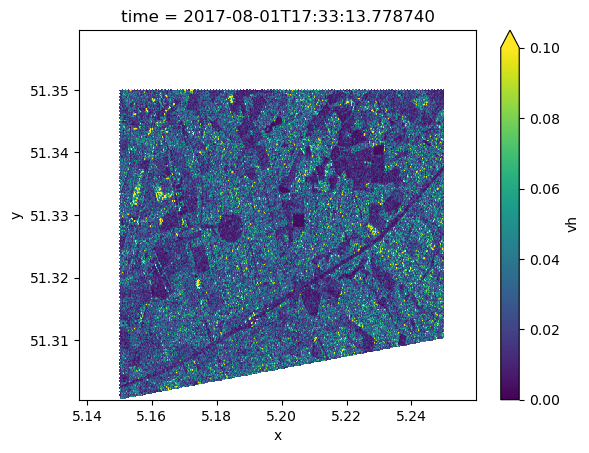

Radar Vegetation Index¶

Now that we have our geocoded GRD data, we can compute the vegetation indexes:

Radar Vegetation Index (RVI) by Nasirzadehdizaji et al.: $RVI = \frac{4\sigma^0_{VH}}{\sigma^0_{VV}+\sigma^0_{VH}}$
Dual-pol Radar Vegetation Index for GRD data (DpRVI) by Bhogapurapu et al.: $DpRVI = \frac{q(q+3)}{(q+1)^2}$ where $q = \frac{\sigma^0_{VH}}{\sigma^0_{VV}}$

RVI = 4 * ds.vh / (ds.vv + ds.vh)

q = ds.vh / ds.vv
DpRVI = q * (q + 3) / (q + 1) ** 2

Time Series Analysis¶

We were able to compute the indexes for a single step in time. However a single view is not enough to characterize the vegetation behaviour in the long term.
Therefore, we have to do the same processing for all the products we selected via the STAC API.

from joblib import Parallel, delayed


def preprocess_grd(grd_path, bbox):
    # Data Access
    dt = xr.open_datatree(grd_path, engine="zarr", chunks="auto")
    t = np.datetime64(dt.attrs["stac_discovery"]["properties"]["datetime"][:-2], "ns")

    group_VH = [x for x in dt.children if "VH" in x][0]
    grd = dt[group_VH].measurements.to_dataset().rename({"grd": "vh"})
    group_VV = [x for x in dt.children if "VV" in x][0]
    grd["vv"] = dt[group_VV].measurements.to_dataset().grd

    # Spatial Slicing
    gcps = dt[group_VH].conditions.gcp.to_dataset()[["latitude", "longitude"]]
    mask = (
        (gcps.latitude < bbox[3])
        & (gcps.latitude > bbox[1])
        & (gcps.longitude < bbox[2])
        & (gcps.longitude > bbox[0])
    )
    idx = np.where(mask == 1)
    if len(idx[0]) == 0 or len(idx[1]) == 0:
        return None
    azimuth_time_slice, ground_range_slice = build_slice(mask.shape, idx)

    gcps_crop = gcps.isel(
        dict(azimuth_time=azimuth_time_slice, ground_range=ground_range_slice)
    )

    azimuth_time_min = gcps_crop.azimuth_time.min().values
    azimuth_time_max = gcps_crop.azimuth_time.max().values

    ground_range_min = gcps_crop.ground_range.min().values
    ground_range_max = gcps_crop.ground_range.max().values

    grd_crop = grd.sel(
        dict(
            azimuth_time=slice(azimuth_time_min, azimuth_time_max),
            ground_range=slice(ground_range_min, ground_range_max),
        )
    )

    gcps_crop_interp = gcps_crop.interp_like(grd_crop)
    grd_crop = grd_crop.assign_coords(
        {"latitude": gcps_crop_interp.latitude, "longitude": gcps_crop_interp.longitude}
    )
    mask_2 = (
        (gcps_crop_interp.latitude < bbox[3])
        & (gcps_crop_interp.latitude > bbox[1])
        & (gcps_crop_interp.longitude < bbox[2])
        & (gcps_crop_interp.longitude > bbox[0])
    )
    grd_crop = grd_crop.where(mask_2.compute(), drop=True)

    # Calibration

    sigma_lut = dt[group_VH].quality.calibration.sigma_nought

    sigma_lut_line_pixel = xr.DataArray(
        data=sigma_lut.data,
        dims=["line", "pixel"],
        coords=dict(
            line=(["line"], sigma_lut.line.values),
            pixel=(["pixel"], sigma_lut.pixel.values),
        ),
    )
    grd_line_pixel = xr.DataArray(
        data=grd_crop.vh.data,
        dims=["line", "pixel"],
        coords=dict(
            line=(["line"], grd_crop.vh.line.values),
            pixel=(["pixel"], grd_crop.vh.pixel.values),
        ),
    )
    sigma_lut_interp_line_pixel = sigma_lut_line_pixel.interp_like(
        grd_line_pixel, method="linear"
    )

    sigma_lut_interp = xr.DataArray(
        data=sigma_lut_interp_line_pixel.data,
        dims=["azimuth_time", "ground_range"],
        coords=dict(
            azimuth_time=(["azimuth_time"], grd_crop.azimuth_time.values),
            ground_range=(["ground_range"], grd_crop.ground_range.values),
        ),
    )

    sigma_0 = (abs(grd_crop.astype(np.float32)) ** 2) / (sigma_lut_interp**2)
    sigma_0 = sigma_0.assign_coords(time=t)

    return [
        sigma_0,
        (
            np.min(sigma_0.latitude.values).item(),
            np.max(sigma_0.latitude.values).item(),
        ),
        (
            np.min(sigma_0.longitude.values).item(),
            np.max(sigma_0.longitude.values).item(),
        ),
    ]


grd_products = Parallel(n_jobs=-1)(
    delayed(preprocess_grd)(grd_path, bbox) for grd_path in grd_paths
)

Extract min/max values for the longitude and latitude to build a common regular grid

min_lat = np.min([i[1][0] for i in grd_products if i is not None])
max_lat = np.max([i[1][1] for i in grd_products if i is not None])

min_lon = np.min([i[2][0] for i in grd_products if i is not None])
max_lon = np.max([i[2][1] for i in grd_products if i is not None])

grid_x_regular, grid_y_regular = create_regular_grid(
    min_lon, max_lon, min_lat, max_lat, 0.0001
)

Geocode and combine the time series of sigma nought data into a single datacube:

grd_products_geocoded = Parallel(n_jobs=-1)(
    delayed(geocode_grd)(grd_product[0], grid_x_regular, grid_y_regular)
    for grd_product in grd_products
    if grd_product is not None
)
sigma_0_series = xr.concat(grd_products_geocoded, dim="time").sortby("time")

Combine data from adjacent GRD scenes for the same day (coming from different Zarr products):

sigma_0_series = (
    sigma_0_series.groupby("time.date").max("time").rename(dict(date="time"))
)
sigma_0_series

sigma_0_series = sigma_0_series.where(~np.isnan(sigma_0_series), drop=True)

Store the result locally, so that in case the Kernel crashes it will be possible to start again from the next cell, skipping the pre-processing steps.

sigma_0_series["time"] = [pd.to_datetime(x) for x in sigma_0_series.time.values]
sigma_0_series.to_zarr("sigma_0_series.zarr", mode="w")

<xarray.backends.zarr.ZarrStore at 0x7f228417c540>

import xarray as xr

sigma_0_series = xr.open_dataset("sigma_0_series.zarr", engine="zarr")

Compute the vegetation indexes:

ds = sigma_0_series

RVI = (4 * ds.vh) / (ds.vv + ds.vh)

q = ds.vh / ds.vv
DpRVI = q * (q + 3) / (q + 1) ** 2

Spatial Aggregation¶

A sample geoJSON file containing the field of three different crop fields boundaries provides us the location of interest to perform our analysis:

import geopandas as gpd

fields = gpd.read_file("./geojson/fields.geojson")
fields

We can visualize the overlay the field boundaries with the geocoded backscatter:

import matplotlib.pyplot as plt
import cartopy.crs as ccrs

plt.figure(figsize=(16, 8))
ax = plt.subplot(projection=ccrs.PlateCarree())
sigma_0_series.vh[0].plot.imshow(vmin=0, vmax=0.1, ax=ax)
fields.plot(ax=ax, color="red")

<GeoAxes: title={'center': 'time = 2017-05-03'}, xlabel='x', ylabel='y'>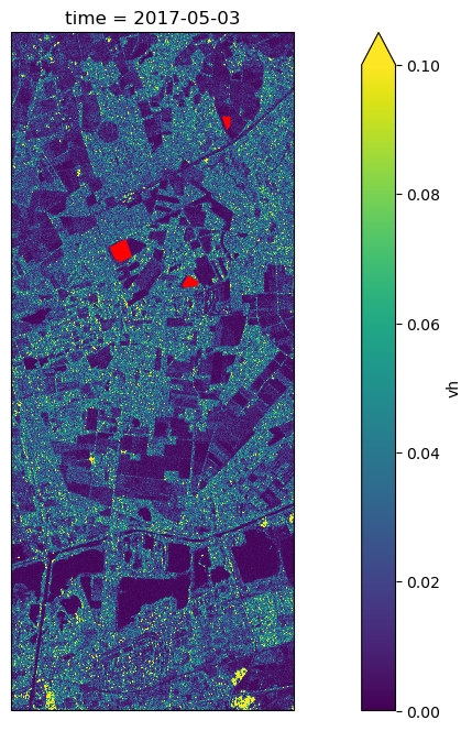

Now we can use the Xvec library to aggregate our radar vegetation index values over the specific fields:

aggregated_DpRVI = DpRVI.xvec.zonal_stats(fields.geometry, x_coords="x", y_coords="y")
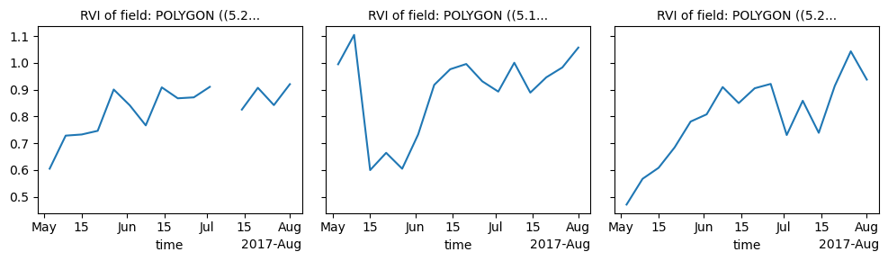
aggregated_RVI = RVI.xvec.zonal_stats(fields.geometry, x_coords="x", y_coords="y")

And finally plot the resulting time series. We will notice that the two variations of the radar vegetation index assume really similar values, where the main difference is that the DpRVI is scaled between 0 and 1, whereas the RVI is not.

ax0 = aggregated_DpRVI.plot(col="geometry", col_wrap=3)
ax0.set_titles("DpRVI of field: {value}")
ax1 = aggregated_RVI.plot(col="geometry", col_wrap=3)
ax1.set_titles("RVI of field: {value}")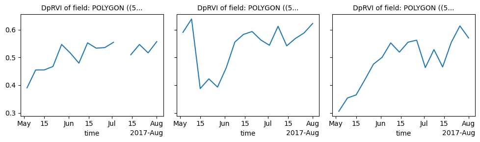

Summary¶

This notebook showed a complete Sentinel-1 GRD pipeline: from the data access to the final time series analysis.

Some important remarks:

Sentinel-1 GRD data has to be calibrated and geocoded before using it in this kind of analysis.
This notebook proposes an efficient way to crop and geocode the data, which is highly relevant for small areas and long time series.

Welcome

Sentinel-1 L2 OCN Zarr Product Exploration

Welcome

STAC-Based Exploration and Visualization of Sentinel-2 and Sentinel-1 Data