Wildfire Burn Severity Assessment Using Sentinel-2 L2A Data and dNBR
A hands-on tutorial using EOPF STAC Zarr datasets, Dask and Xarray to map and quantify burnt areas for the Peneda-Gerês wildfire event (Portugal, July 2025).

Table of Contents
Run this notebook interactively with all dependencies pre-installed
Introduction
Wildfires are one of the most destructive natural hazards affecting ecosystems, biodiversity, and local communities. For Earth Observation (EO)-based wildfire impact assessment, it is essential to define appropriate temporal ranges before and after the event to analyse vegetation conditions, burned area characteristics, and severity using indices such as Normalised Burn Ratio(NBR) and delta NBR(dNBR).
In this notebook, we focus on the Peneda-Gerês / Ponte da Barca wildfire, located in the north-western region of Portugal, close to the border with Spain. This area is part of the Peneda-Gerês National Park, a region with dense forest cover and rich ecological value, making it a critical location for post-fire environmental monitoring.
We analyse multi-temporal Sentinel-2 L2A imagery covering:
Event date → 2025-07-26
± 1 month window around the fire event
Extended pre- and post-event periods to study vegetation recovery
Justification for Temporal and Spatial Bounds
Temporal Window Justification
For this analysis we selected a one-month pre-fire and one-month post-fire comparison window, rather than a 15-day range. Using a longer time window helps reduce the influence of short-term atmospheric variations, cloud cover issues, and rapid phenological changes common in the summer season.
The defined periods are:
Event date (Ignition date): 2025-07-26
Week before event: 2025-07-19
Week after event: 2025-08-02
Pre-event period: 2025-06-20 → 2025-07-19
Post-event period: 2025-08-02 → 2025-09-02
Why 1-month windows?
Using a 30-day window before and after the wildfire ensures:
Stable baseline vegetation conditions for comparison — reducing noise due to daily fluctuations.
Greater probability of cloud-free Sentinel-2 acquisitions, improving the reliability of pre/post composite images.
Better representation of ecological response, as vegetation recovery or burn scar persistence is visible over weeks, not days.
Alignment with wildfire monitoring standards, where analytical best practice recommends at least ~1 month around the fire for robust burn severity and vegetation-change evaluation.
A shorter ±15-day period may miss key signals because:
Sentinel-2 revisit time (5 days per tile but impacted by cloud cover) can limit usable scenes,
Vegetation stress and burn severity spectral response evolve across several weeks.
Thus, the 1-month buffer enables more accurate dNBR burn scar quantification.
Spatial Extent Justification
The region of interest covers the Peneda-Gerês / Ponte da Barca wildfire zone, located in north-west Portugal on the border with Spain. This AOI fully encompasses the reported burn perimeter and surrounding vegetation for comparison. The selected spatial boundary:
Captures the entire affected ecosystem within the Peneda-Gerês National Park,
Includes buffer land surrounding the burn to analyze edge effects and severity gradients,
Minimizes processing cost by avoiding unnecessary surrounding territory.
This spatial coverage is ecologically and operationally important because:
Peneda-Gerês is Portugal’s only national park and a biodiversity hotspot,
The region shares a transboundary forest system with Spain,
Dense vegetation and rugged topography accelerate fire spread and intensify burn patterns.
Together, the temporal and spatial definitions provide a scientifically justified foundation for a comprehensive wildfire impact assessment using Sentinel-2 L2A imagery.
Overview
Setup
Start importing the necessary libraries
from dask_gateway import Gateway

from xcube.core.store import new_data_store
from xcube_resampling.utils import reproject_bbox
Create and Startup Dask Cluster
Create Local Dask Cluster to access and process the data in parallel.
# Simplest way - creates everything automatically in the eopf jupyterhub dask cluster
gate = Gateway()
cluster = gate.new_cluster()Analysing in Detail
Now that we have an idea of a potential wildfire event, we can explore in a bit more detail to see what areas where affected most.
We will use higher resolution sentinel-2-l2a data to compute the Normalised Burn Ratio (NBR) index to highlight burned areas. The NBR index uses near-infrared (NIR) and shortwave-infrared (SWIR) wavelengths. We will use xcube-eopf package to search and extract required data for cloud free days.
To estimate the amount of burnt area we will compute the difference between the NBR from period before the fire date and the NBR from the period after. The first step is to select the week before and the week after the wildfire.
Pre-Event Data Preparation
store = new_data_store("eopf-zarr")
bbox_4326 = [-8.375, 41.700, -8.075, 41.875]
crs_utm = "EPSG:32629"
bbox_utm = reproject_bbox(bbox_4326, "EPSG:4326", crs_utm)
prefire_ds = store.open_data(
    data_id="sentinel-2-l2a",
    bbox=bbox_utm,
    time_range=["2025-06-20", "2025-07-19"],
    spatial_res=10,
    crs=crs_utm,
    variables=["b08", "b12"],
    query={"eo:cloud_cover": {"lt": 20}},
)
print(prefire_ds)
prefire_ds = prefire_ds.mean(dim="time")
prefire_ds
<xarray.Dataset> Size: 553MB
Dimensions: (time: 7, y: 1967, x: 2511)
Coordinates:
* time (time) datetime64[ns] 56B 2025-06-20T11:33:19.024000 ... 202...
spatial_ref int64 8B ...
* x (x) float64 20kB 5.519e+05 5.519e+05 ... 5.77e+05 5.77e+05
* y (y) float64 16kB 4.636e+06 4.636e+06 ... 4.617e+06 4.617e+06
Data variables:
b08 (time, y, x) float64 277MB dask.array<chunksize=(1, 1830, 1830), meta=np.ndarray>
b12 (time, y, x) float64 277MB dask.array<chunksize=(1, 1830, 1830), meta=np.ndarray>
Attributes: (4)
Post-Event Data Preparation
store = new_data_store("eopf-zarr")
bbox_4326 = [-8.375, 41.700, -8.075, 41.875]
crs_utm = "EPSG:32629"
bbox_utm = reproject_bbox(bbox_4326, "EPSG:4326", crs_utm)
postfire_ds = store.open_data(
    data_id="sentinel-2-l2a",
    bbox=bbox_utm,
    time_range=["2025-08-02", "2025-09-02"],
    spatial_res=10,
    crs=crs_utm,
    variables=["b08", "b12"],
    query={"eo:cloud_cover": {"lt": 20}},
)
print(postfire_ds)
postfire_ds = postfire_ds.mean(dim="time")
postfire_ds
<xarray.Dataset> Size: 948MB
Dimensions: (time: 12, y: 1967, x: 2511)
Coordinates:
* time (time) datetime64[ns] 96B 2025-08-03T11:21:31.024000 ... 202...
spatial_ref int64 8B ...
* x (x) float64 20kB 5.519e+05 5.519e+05 ... 5.77e+05 5.77e+05
* y (y) float64 16kB 4.636e+06 4.636e+06 ... 4.617e+06 4.617e+06
Data variables:
b08 (time, y, x) float64 474MB dask.array<chunksize=(1, 1830, 1830), meta=np.ndarray>
b12 (time, y, x) float64 474MB dask.array<chunksize=(1, 1830, 1830), meta=np.ndarray>
Attributes: (4)
Calculating the NBR Index
In the next step we will calculate our index, using simple band math. We first define a function that calculates our index given a dataset with nir/swir22 band data and then add the additional variable to our pre-fire/post-fire datasets.
index_name = "NBR"


# Normalised Burn Ratio, Lopez Garcia 1991
def calc_nbr(ds):
    return (ds.b08 - ds.b12) / (ds.b08 + ds.b12)


index_dict = {index_name: calc_nbr}

prefire_ds[index_name] = index_dict[index_name](prefire_ds)
postfire_ds[index_name] = index_dict[index_name](postfire_ds)
Now that we have the indecies calculated we can calculate the difference in burnt area between the two periods to analyse which regions have been burnt.
Note that at this point we haven’t actually loaded the data or done the calculations, we’ve just defined a task graph for dask to execute. When we call persist() the graph up to that point will be executed and the data saved for in the distributed memory of our workers. We do this at this stage to avoid fetching the data multiple times in future computations.
We then save our result (which is a dataarray) in a new dataset: dnbr_dataset.
# calculate delta NBR
prefire_burnratio = (
    prefire_ds.NBR.persist()
)  # <--- load and keep data into your workers
postfire_burnratio = (
    postfire_ds.NBR.persist()
)  # <--- load and keep data into your workers

delta_NBR = prefire_burnratio - postfire_burnratio

dnbr_dataset = delta_NBR.to_dataset(name="delta_NBR").compute()
Plotting and Visualization
We will now plot our data from before, after and the delta of our wildfire event to further analyse.
Plotting Before
prefire_burnratio.plot()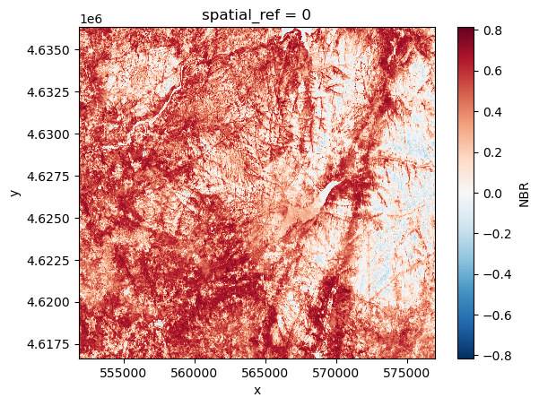
Plotting After
postfire_burnratio.plot()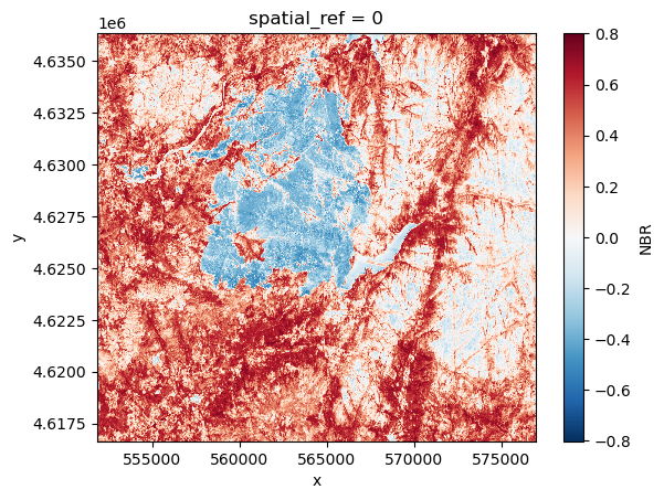
Plotting Delta
The plot below highligths the burnt regions.
dnbr_dataset.delta_NBR.plot()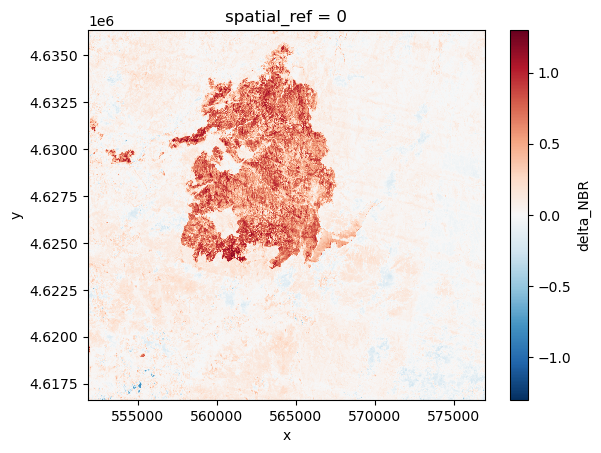
Analysing Burnt Areas
Great, now that we’ve calculated the delta NBR (dNBR), we can estimate the amount of area that was burned. First we need to classify which pixels are actually burned and then calculate the area that was burned.
To classify burned area we can use the dNBR reference ratio ratios described in: https://
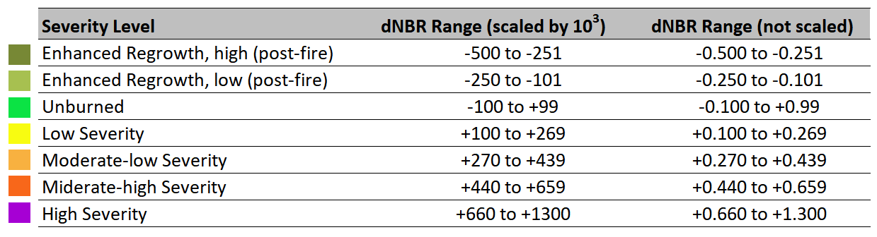
BURN_THRESH = 0.440
burn_mask = (
    dnbr_dataset.delta_NBR > BURN_THRESH
)  # True/False mask, same shape as raster
burn_mask.plot()

# save the burn_mask to our dataset
dnbr_dataset["burned_ha_mask"] = burn_mask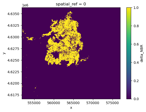
Burnt Area
Now with the above a data mask where all pixels classified as burnt are 1 and the non burnt ones are 0. To calculate burnt area, we simply sum all pixels and multiply them by the area which a pixel covers (i.e. the resolution, which in our case is 10m/p).
At the same step we will convert our metric to hectares (ha).
# dx, dy = dnbr_dataset.delta_NBR.rio.resolution()
dx = 10.0
dy = -10.0
pixel_area_ha = abs(dx * dy) / 1e4  # 10m × 10m = 0.01 ha

pixels_burnt = burn_mask.sum().compute().item()  # integer number of burnt pixels
burnt_area_ha = pixels_burnt * pixel_area_ha

print(f"Burnt area   : {burnt_area_ha:,.2f} ha")
Burnt area : 5,506.85 ha
cluster.close()Links and Refernces
https://
www .sciencedirect .com /science /article /pii /S1470160X22004708 #f0035 https://
un -spider .org /advisory -support /recommended -practices /recommended -practice -burn -severity /in -detail /normalized -burn -ratio](https:// un -spider .org /advisory -support /recommended -practices /recommended -practice -burn -severity /in -detail /normalized -burn -ratio https://
corteva .github .io /rioxarray /stable /examples /reproject _match .html
