Building Sentinel-3 Data Cubes with xcube EOPF

Table of Contents¶

1. Introduction
2. Install the xcube-eopf Data Store
3. Main Features of the xcube-eopf Data Store for Sentinel-3
4. Import modules
5. Open multiple Sentinel-3 samples as anaylsis-ready data cube
6. Conclusion

Introduction¶

xcube-eopf is a Python package and xcube plugin that adds a data store named eopf-zarr to xcube. The data store is used to provide analysis-ready datacubes (ARDC) from EOPF Sentinel Zarr Samples.

This notebook demonstrates how to use the xcube-eopf plugin to explore and analyze EOPF Sentinel Zarr Samples. It highlights the key features currently supported by the plugin.

• 🐙 GitHub: EOPF Sample Service – xcube-eopf
• ❗ Issue Tracker: Submit or view issues
• 📘 Documentation: xcube-eopf Docs

Install the xcube-eopf Data Store¶

The xcube-eopf package is implemented as a xcube plugin and can be installed using either pip or conda/mamba from the conda-forge channel.

• 📦 PyPI: xcube-eopf on PyPI pip install xcube-eopf

• 🐍 Conda (conda-forge): xcube-eopf on Anaconda conda install -c conda-forge xcube-eopf

  You can also use Mamba as a faster alternative to Conda: mamba install -c conda-forge xcube-eopf

Main Features of the xcube-eopf Data Store for Sentinel-3¶

The xcube-eopf plugin uses the xarray-eopf backend to access individual EOPF Zarr samples, then leverages xcube’s data processing capabilities to generate a 3D analysis-ready datacube (ARDCs) from multiple samples.

Currently, this functionality supports Sentinel-2 and Sentinel-3 products.

The EOPF xcube data store so far supports three Sentinel-3 product types via the data_id argument:

Data Cube Generation Workflow

The workflow for building 3D analysis-ready cubes from Sentinel-3 products involves the following steps, which are implemented in the open_data() method:

1. Query tiles using the EOPF Zarr Sample Service STAC API for a given time range and spatial extent.
2. Group items by solar day.
3. Rectify data from the native 2D irregular grid to a regular grid using xcube-resampling.
4. Mosaic adjacent tiles into seamless daily scenes.
5. Stack the daily mosaics along the temporal axis to form 3D data cubes for each variable (e.g., spectral bands).

📚 More info: xcube-eopf Documentation

Import Modules¶

The xcube-eopf data store is implemented as a plugin for xcube. Once installed, it registers the store ID eopf-zarr automatically and a new data store instance can be initiated via xcube’s new_data_store() method.

We can list all avaialbe data ids with corresponds to the collection of the STAC catalog.

Open Multiple Sentinel-3 Samples as an Analysis-Ready Data Cube¶

The open_data() method allows you to open multiple Sentinel-3 samples as a single, analysis-ready data cube.

Each supported data product has its own set of parameters. You can retrieve detailed descriptions of these parameters — including their format and whether they are required — using the get_open_data_params_schema() function.

Below the opening parameters for the Sentinel-2 product (applicable for L1C and L2A) are summarized:

Required parameters:

• bbox: Bounding box [“west”, “south”, “est”, “north”] in CRS coordinates.
• time_range: Temporal extent [“YYYY-MM-DD”, “YYYY-MM-DD”].
• spatial_res: Spatial resolution in meter of degree (depending on the CRS).
• crs: Coordinate reference system (e.g. "EPSG:4326").

These parameters control the STAC API query and define the output cube’s spatial grid.

Optional parameters:

• variables: Variables to include in the dataset. Can be a name or regex pattern or iterable of the latter.
  • sentinel-3-olci-l1-efr: oa01_radiance, oa02_radiance, oa03_radiance, oa04_radiance, oa05_radiance, oa06_radiance, oa07_radiance, oa08_radiance, oa09_radiance, oa10_radiance, oa11_radiance, oa12_radiance, oa13_radiance, oa14_radiance, oa15_radiance, oa16_radiance, oa17_radiance, oa18_radiance, oa19_radiance, oa20_radiance, oa21_radiance
  • sentinel-3-olci-l2-lfr: gifapar, iwv, otci, rc681, rc865
  • sentinel-3-slstr-l2-lst: lst
• tile_size: Spatial tile size of the returned dataset (width, height).
• query: Additional query options for filtering STAC Items by properties. See STAC Query Extension for details.
• interp_methods: Interpolation method(s) for upsampling spatial variables used in xcube_resampling.rectify_dataset
• agg_methods: Aggregation method(s) for downsampling spatial variables. used in xcube_resampling.rectify_dataset

We will now generate an example data cube in a geographic coordinate system using Sentinel-3 SLSTR Level-2 LST and Sentinel-3 OLCI Level-2 LFR products, covering the region of Corsica.

💡 Note
open_data() builds a Dask graph and returns a lazy xarray.Dataset, meaning no variable data is loaded at this stage. However, the rectification algorithm requires the location of each pixel. Therefore, the geoinformation must be downloaded during graph construction to enable rectification.

Now we can request the same data cube but for the Sentinel-3 OLCI Level-2 LFR product.

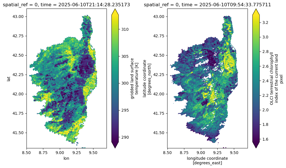
We can plot the SLSTR Land Surface Temperature (lst) and the OLCI Terrestrial Chlorophyll Index (otci, a proxy for chlorophyll content in vegetation) for the first time step as an example. Note that this operation will trigger data downloads and processing.

Conclusion¶

This notebook demonstrates how to open multiple Sentinel-3 products as an analysis-ready data cube using the xcube-eopf data store. Below is a summary of the key takeaways:

• 3D analysis-ready spatio-temporal data cubes can be generated from multiple EOPF Sentinel-3 Zarr samples for the following collections:
  • sentinel-3-olci-l1-efr
  • sentinel-3-olci-l2-lfr
  • sentinel-3-slstr-l2-lst
• The cube generation workflow follows this pattern:
  1. Query tiles using the EOPF Zarr Sample Service STAC API for a given time range and spatial extent.
  2. Group items by solar day.
  3. Rectify data from the native 2D irregular grid to a regular grid using xcube-resampling.
  4. Mosaic adjacent tiles into seamless daily scenes.
  5. Stack the daily mosaics along the temporal axis to form 3D data cubes for each variable (e.g., spectral bands).

Future Development¶

• Extend support to include Sentinel-1 data.
• Continue active development of the plugin through January 2026, at least within the scope of the EOPF Sentinel Zarr Samples project.