SENTINEL-1 L1 GRD Product Format Prototype¶

Table of Contents¶

Introduction
Import modules
File path definition
Read local files with EOPF
Read remote files with xarray-datatree
Examples of product usage
A. Decimation data
B. Geocoding using GCPs
C. Geographic selection

Introduction¶

In this notebook we will show an example of grd TOPSAR product and some easy usage examples

Objectives:

Provide ready-to-use datasets and data variable
Allow users to open and manipulate data using both standard external tools and the EOPF

Relevant Features:

Swaths, bursts and polarization are separeted in different products
The coordinates associated to the data are the physical coordinates
The zarr product will adhere to CF convetion (this allow the user to open the prodoct with standards tools, such as xarray, exploiting properly the data coordinates).

Notes:

It is a preliminary example of product

Not all the metadata are included in these product prototype, but they will be included in the future.
Among the excluded metadata, there are:
- RFI
- qualityInformation
- downlinkInformation
The stac attrabutes are still to be defined.
The name of the variables are preliminary and they may change in the future.
Variable attributes will be refined in the future, including:
- long_name
- units
- and standard names for coordinates
The chunking is not defined yet.
Products naming convention is to be defined.
Reading from local and remote storage with EOPF is experimental(branch feat/coords_in_vars, commit 10a4f2e1) and not officially released.1) and not offically released.

Import modules¶

Dependencies

datatree
eopf
xarray
matplotlib
cartopy

%matplotlib inline

import datatree
import xarray as xr

import matplotlib.pyplot as plt

plt.rcParams["figure.figsize"] = (10, 5)
plt.rcParams["font.size"] = 10

File path definition¶

GRD: S1A_IW_GRDH_1SDV_20240201T164915_20240201T164940_052368_065517_750E

polarization:VH

Remote file path

remote_product_path = "https://storage.sbg.cloud.ovh.net/v1/AUTH_8471d76cdd494d98a078f28b195dace4/sentinel-1-public/demo_product/grd/S01SIWGRH_20240201T164915_0025_A146_S000_5464A_VH.zarr"

Local file

The listed file do not work with the latest eopf-cpm library and therefore the next cells are commented out

# # Download the files into the folder ./scratch/demo_product/grd/
# !mkdir -p ./scratch/demo_product/
# !wget -q -r -nc -nH --cut-dirs=5 https://storage.sbg.cloud.ovh.net/v1/AUTH_8471d76cdd494d98a078f28b195dace4/sentinel-1-public/demo_product/grd/ --no-parent -P ./scratch/demo_product/grd/ --reject "index.html*"

# # Set the local product paths using the specified directory
# local_product_path = "./scratch/demo_product/grd/S01SIWGRH_20240201T164915_0025_A146_S000_5464A_VH.zarr"

Read local files with EOPF¶

# store = EOZarrStore('./scratch/demo_product/grd/S01SIWGRH_20240201T164915_0025_A146_S000_5464A_VH.zarr')
# store = store.open()
# product = store.load()

# product

Read remote files with xarray-datatree¶

(xarray extension that allow performing operations on hierachical structures)

dt = datatree.open_datatree(remote_product_path, engine="zarr", chunks={})
dt

Examples of product usage¶

# open data with xarray
grd = xr.open_dataset(remote_product_path, group="measurements", engine="zarr")["grd"]

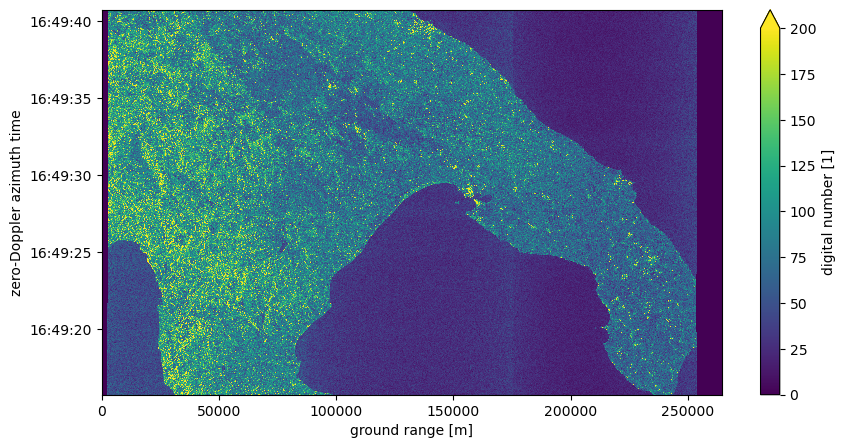
Decimation data¶

## decimation
grd_decimated = grd.isel(
    azimuth_time=slice(None, None, 10), ground_range=slice(None, None, 10)
)

## plot
grd_decimated.plot(vmax=200)
plt.show()

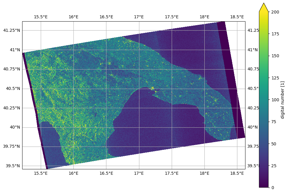
Geocoding using GCPs¶

Interpolate and assign new geographic coordinates

gcp = xr.open_dataset(remote_product_path, group="conditions/gcp", engine="zarr")
gcp_iterpolated = gcp.interp_like(grd_decimated)

grd_decimated = grd_decimated.assign_coords(
    {"latitude": gcp_iterpolated.latitude, "longitude": gcp_iterpolated.longitude}
)

Plot in geographic coordinates

import cartopy.crs as ccrs

_, ax = plt.subplots(subplot_kw={"projection": ccrs.Miller()}, figsize=(12, 8))
gl = ax.gridlines(
    draw_labels=True, crs=ccrs.PlateCarree(), x_inline=False, y_inline=False
)
grd_decimated.plot(
    ax=ax, transform=ccrs.PlateCarree(), x="longitude", y="latitude", vmax=200
)
plt.show()

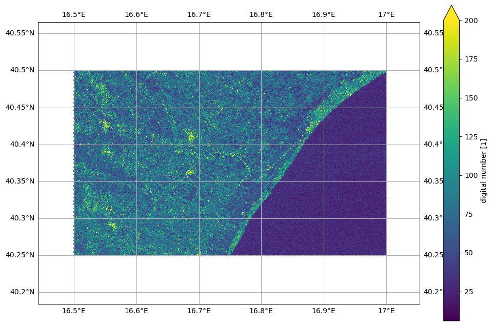
Geographic selection¶

Region definition

lat_max = 40.5
lat_min = 40.25
lon_max = 17
lon_min = 16.5

polygon_lon = [lon_min, lon_max, lon_max, lon_min, lon_min]
polygon_lat = [lat_max, lat_max, lat_min, lat_min, lat_max]

Crop using lon lat coordinates

mask = (
    (grd_decimated.latitude < lat_max)
    & (grd_decimated.latitude > lat_min)
    & (grd_decimated.longitude < lon_max)
    & (grd_decimated.longitude > lon_min)
)
grd_crop = grd_decimated.where(mask, drop=True)

Plot in geographic coordinates

_, ax = plt.subplots(subplot_kw={"projection": ccrs.Miller()}, figsize=(12, 8))
gl = ax.gridlines(
    draw_labels=True, crs=ccrs.PlateCarree(), x_inline=False, y_inline=False
)
grd_decimated[::5, ::5].plot(
    ax=ax,
    transform=ccrs.PlateCarree(),
    x="longitude",
    y="latitude",
    vmax=200,
)
plt.plot(
    polygon_lon,
    polygon_lat,
    color="red",
    linewidth=2,
    marker="o",
    transform=ccrs.PlateCarree(),
)


_, ax = plt.subplots(subplot_kw={"projection": ccrs.Miller()}, figsize=(12, 8))
gl = ax.gridlines(
    draw_labels=True, crs=ccrs.PlateCarree(), x_inline=False, y_inline=False
)
grd_crop.plot(
    ax=ax,
    transform=ccrs.PlateCarree(),
    x="longitude",
    y="latitude",
    vmax=200,
)
plt.show()

Jupyter Notebooks

Sentinel-2 L1C MSI Zarr Product Exploration

Jupyter Notebooks

SENTINEL-1 L1 SLC TOPSAR Product Format Prototype