Example for xarray and xcube

Author(s): Konstantin Ntokas
Affiliation: Brockmann Consult
Contact: konstantin.ntokas@brockmann-consult.de

Introduction¶

This notebook demonstrates the features of the xarray EOPF backend and the xcube EOPF data store.

Questions:

How can EOPF Zarr samples be opened in an analysis-ready data model?
How can 3D data cubes be generated from EOPF Zarr samples?

Objectives:

Understand the key features of the xarray EOPF backend, including its analysis-ready mode.
Learn how to use the xcube EOPF data store to open multiple Sentinel EOPF Zarr samples and combine them into a 3D data cube.

Disclaimer
This notebook demonstrates the use of open source software and is intended for educational and illustrative purposes only. All software used is subject to its respective licenses. The authors and contributors of this notebook make no guarantees about the accuracy, reliability, or suitability of the content or included code. Use at your own discretion and risk. No warranties are provided, either express or implied.

Table of Contents¶

🔹 Setup
🔹 xarray EOPF backend: Open one Sample
🔹 xcube EOPF data store: Open multiple Sample
🔹 Conclusion

Setup¶

The xarray EOPF backend and xcube EOPF backend are implemented as an xarray plugin and xcube plugin, respectively. Both can be installed using either pip or conda/mamba from the conda-forge channel.

📦 PyPI: pip install xarray-eopf and pip install xcube-eopf
🐍 Conda (conda-forge): conda install -c conda-forge xarray-eopf and conda install -c conda-forge xcube-eopf

You can also use Mamba as a faster alternative to Conda: mamba install -c conda-forge xarray-eopf

import os

import matplotlib.colors as mcolors
import matplotlib.pyplot as plt
import numpy as np
import pystac_client
import xarray as xr
from xcube.core.store import new_data_store
from xcube.webapi.viewer import Viewer
from xcube_eopf.utils import reproject_bbox

xarray EOPF backend: Open one Sample¶

The xarray-eopf backend for EOPF data products can be selecterd by setting engine="eopf-zarr" in xarray.open_dataset(..) and xarray.open_datatree(..) method. It supports two modes of operation:

Analysis Mode (default)
Native Mode

Native mode¶

We can use the EOPF Zarr Samples STAC API to search for tiles by bounding box and time range.
The "product" asset can be used to open an EOPF Zarr product.
Additional fields in the asset provide the parameters required to open the dataset.

catalog = pystac_client.Client.open("https://stac.core.eopf.eodc.eu")
items = list(
    catalog.search(
        collections=["sentinel-2-l2a"],
        bbox=[7.2, 44.5, 7.4, 44.7],
        datetime=["2025-04-30", "2025-05-01"],
    ).items()
)
items

[<Item id=S2B_MSIL2A_20250430T101559_N0511_R065_T32TLQ_20250430T131328>]

We can now use the href and xarray:open_datatree_kwargs from the item to open the product.

item = items[0]
href = item.assets["product"].href
open_params = item.assets["product"].extra_fields["xarray:open_datatree_kwargs"]
open_params

{'chunks': {}, 'engine': 'eopf-zarr', 'op_mode': 'native'}

dt = xr.open_datatree(href, **open_params)
dt

As an example, we plot the quicklook image to view the RGB image.

dt.quality.l2a_quicklook.r60m.tci.plot.imshow(rgb="band")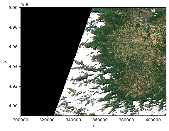

/home/konstantin/micromamba/envs/xcube-eopf/lib/python3.13/site-packages/xcube_resampling/coarsen.py:103: RuntimeWarning: Mean of empty slice
  return nan_reducer(block, axis)

The same applies to the xr.open_dataset method, which returns a flattened DataTree represented as an xr.Dataset.

Note, this mode can be usefull to support compatibility with existing workflows that rely on the traditional xr.Dataset model, since the xarray.DataTree data model is relatively new, introduced in xarray v2024.10.0 (October 2024).

ds = xr.open_dataset(
    item.assets["product"].href,
    **item.assets["product"].extra_fields["xarray:open_datatree_kwargs"]
)
ds

We can also filter the output variables indicated as string, an iterable of names, or a regular expression (regex) pattern, as shown below.

ds = xr.open_dataset(
    item.assets["product"].href,
    **item.assets["product"].extra_fields["xarray:open_datatree_kwargs"],
    variables="measurements*"
)
ds

Analysis Mode¶

The analysis mode provides an analysis-ready, resampled view of the data, currently available for Sentinel-2 and Sentinel-3.

In-depth examples:

ds = xr.open_dataset(
    href, engine="eopf-zarr", chunks={}, op_mode="analysis", resolution=60
)
ds

fig, ax = plt.subplots(1, 2, figsize=(12, 5))

ds.b08.plot(ax=ax[0], robust=True)
ax[0].set_title("B08 (NIR)")

cmap = mcolors.ListedColormap(ds.scl.attrs["flag_colors"].split(" "))
nb_colors = len(ds.scl.attrs["flag_values"])
norm = mcolors.BoundaryNorm(
    boundaries=np.arange(nb_colors + 1) - 0.5, ncolors=nb_colors
)
im = ds.scl.plot.imshow(ax=ax[1], cmap=cmap, norm=norm, add_colorbar=False)
cbar = fig.colorbar(im, ax=ax[1], ticks=ds.scl.attrs["flag_values"])
cbar.ax.set_yticklabels(ds.scl.attrs["flag_meanings"].split(" "))
cbar.set_label("Class")
ax[1].set_title("Scene classification layer")

plt.tight_layout()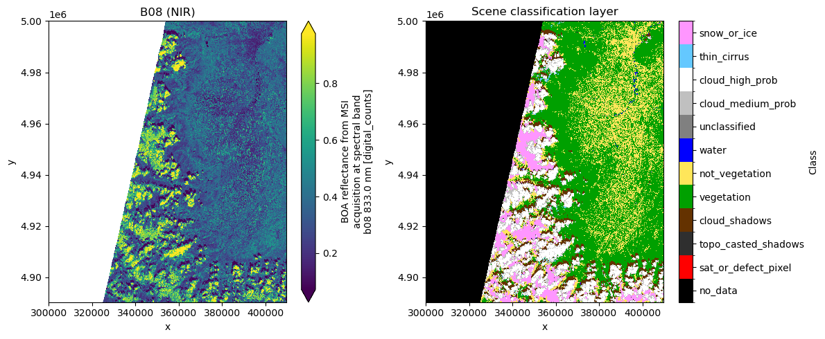

xcube EOPF data store: Open multiple Sample¶

This plugin allows to generate 3D spatiotemporal datacubes from multiple EOPF Zarr Samples. The workflow for building these data cubes involves the following steps:

Query products using the EOPF STAC API for a given time range and spatial extent.
Retrieve observations as cloud-optimized Zarr chunks via the xarray-eopf backend.
Mosaic spatial tiles into single images per timestamp.
Stack the mosaicked scenes along the temporal axis to form a 3D cube.

In-depth examples:

The workflow is integrated into the open_data method, with is shown below. First we need to create data store instance.

store = new_data_store("eopf-zarr")

bbox = [9.85, 53.5, 10.05, 53.6]
crs_utm = "EPSG:32632"
bbox_utm = reproject_bbox(bbox, "EPSG:4326", crs_utm)

💡 Note
open_data() builds a Dask graph and returns a lazy xarray.Dataset. No actual data is loaded at this point.

%%time
ds = store.open_data(
    data_id="sentinel-2-l2a",
    bbox=bbox_utm,
    time_range=["2025-05-01", "2025-05-07"],
    spatial_res=10,
    crs=crs_utm,
    variables=["b02", "b03", "b04", "scl"],
)
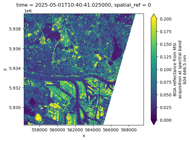
ds

We can plot the the red band (b04) for the first time step as an example. This operation triggers data downloads and processing.

%%time
ds.b04.isel(time=0).plot(vmin=0, vmax=0.2)

CPU times: user 409 ms, sys: 47 ms, total: 456 ms
Wall time: 1.01 s

Now we can request the same data cube but in geographic projection (“EPSG:4326”). xcube-eopf can reproject the datacube to any projection requested by the user.

%%time
ds = store.open_data(
    data_id="sentinel-2-l2a",
    bbox=bbox,
    time_range=["2025-05-01", "2025-05-07"],
    spatial_res=10 / 111320,  # meters converted to degrees (approx.)
    crs="EPSG:4326",
    variables=["b02", "b03", "b04", "scl"],
)
ds

We can load the final data cube into memory, since it is relatively small. This speeds up visualization. For larger data cubes, see the example provided in the xcube-eopf Sentinel-2 notebook available in the gallery.

%%time
ds = ds.persist()

CPU times: user 7.93 s, sys: 1.63 s, total: 9.56 s
Wall time: 4.74 s

Visualization and Analysis¶

💡 Note
If you are running this notebook on the EOPF Sample Service JupyterHub, please set the following environment variable to ensure the Viewer is configured with the correct endpoint.

The environment variable should be set to: "https://jupyterhub.user.eopf.eodc.eu/user/<E-mail>/" Replace <E-mail> with the email address you use to log in to CDSE. This corresponds to the first part of the URL displayed in your browser after logging into JupyterHub.

#os.environ["XCUBE_JUPYTER_LAB_URL"] = "https://jupyterhub.user.eopf.eodc.eu/user/konstantin.ntokas@brockmann-consult.de/"

We can now use xcube Viewer to visualize the cube.

info() gives the URL of the Viewer web application
add_dataset(ds) allows to show the datacube in a Viewer instance in the notebook

viewer = Viewer()
viewer.info()

Server: http://localhost:8000
Viewer: http://localhost:8000/viewer/?serverUrl=http://localhost:8000

404 GET /viewer/config/config.json (127.0.0.1): xcube viewer has not been been configured
404 GET /viewer/config/config.json (127.0.0.1) 16.39ms
501 GET /viewer/state?key=sentinel (127.0.0.1) 0.29ms
404 GET /viewer/ext/contributions (127.0.0.1) 69.00ms

viewer.add_dataset(ds)
viewer.show()

Conclusion¶

This notebook demonstrates the usages of the xarray EOPF backend and the xcube EOPF data store.

Key Takeaways:

xarray EOPF backend offers analysis mode for single product (Sentinel-2 resampling between spectral bands, Sentinel-3 rectification)
xcube EOPF backend allows to open multiple EOPF Zarr samples and build a 3D spatio-temporal datacube:
1. Query via the EOPF STAC API
2. Read using the xarray-eopf backend (Webinar 3)
3. Mosaic along spatial axes
4. Stack along the time axis

Overview

EOPF Zarr Plugins

Overview

Case Study: Wildfire in Sardinia, 2025