Building Sentinel-1 Data Cubes with xcube EOPF Data Store

Table of Contents¶

Introduction
Main Features of the xcube-eopf Data Store for Sentinel-1
Import modules
Access Sentinel-1 Level-1 GRD ARDC
Access Sentinel-1 Level-1 SLC ARDC
Access Sentinel-1 Level-2 OCN ARDC
Conclusion

Run this notebook interactively with all dependencies pre-installed

Introduction¶

xcube-eopf is a Python package that extends xcube with a new data store called "eopf-zarr". This plugin enables the creation of analysis-ready data cubes (ARDC) from multiple Sentinel products published by the EOPF Sentinel Zarr Sample Service.

In this notebook, we demonstrate how to use the xcube EOPF data store to access multiple Sentinel-1 EOPF Zarr products and generate 3D analysis-ready data cubes (ARDC).

For a general introduction to the xcube EOPF Data Store, see the introduction notebook.

🐙 GitHub: EOPF Sample Service – xcube-eopf
❗ Issue Tracker: Submit or view issues
📘 Documentation: xarray-eopf Docs

Main Features of the xcube-eopf Data Store for Sentinel-1¶

Sentinel-1 provides C-band Synthetic Aperture Radar (SAR) data. Unlike optical sensors, SAR actively transmits microwave pulses and measures the returned signal, enabling observations independent of daylight and largely unaffected by cloud cover.

Each pixel measures the radar backscatter, i.e., the fraction of the emitted microwave energy reflected back to the satellite. Bright pixels indicate strong reflections, while dark pixels indicate weak reflections. The measured backscatter depends on factors such as surface roughness, moisture content, geometry, and vegetation structure.

Sentinel-1 supports several radar polarization combinations:

VV – Vertical transmit, Vertical receive
VH – Vertical transmit, Horizontal receive
HH – Horizontal transmit, Horizontal receive
HV – Horizontal transmit, Vertical receive

The available polarization combinations depend on the acquisition mode.

The main Sentinel-1 product types are:

Product	Description	Typical applications	STAC Collection
SLC (Single Look Complex)	Complex-valued radar data (amplitude and phase) in slant-range geometry.	Interferometry (InSAR), ground deformation, DEM generation	sentinel-1-l1-slc
GRD (Ground Range Detected)	Detected radar intensity projected to ground-range geometry. Easier to use than SLC for most applications.	Flood mapping, sea ice, agriculture, ship detection	sentinel-1-l1-grd
OCN (Ocean)	Ocean geophysical products including wind, wave, and surface current information.	Oceanography, marine weather, offshore monitoring	sentinel-1-l2-ocn

Data Cube Generation Workflow¶

STAC query: Retrieve all matching STAC Items based on the requested spatial (bbox) and temporal (time_range) extent.
Grouping: Group the retrieved items by acquisition day, relative orbit, orbit direction (ascending or descending), and satellite platform.
Opening: Open each product in analysis mode using xarray-eopf.
- GRD: Performs radiometric calibration, geocoding based on zero-Doppler geometry using a DEM, and radiometric terrain correction. If no DEM is provided, the Copernicus DEM GLO-30 is automatically retrieved from CDSE. See the GRD documentation.
- SLC: Performs radiometric calibration, TOPSAR burst debursting and merging, geocoding based on zero-Doppler geometry using a DEM, and radiometric terrain correction. If no DEM is provided, the Copernicus DEM GLO-30 is automatically retrieved from CDSE. See the SLC documentation.
- OCN: Rectifies the irregular measurement grid to a regular spatial grid. See the OCN documentation.
Mosaicking: Merge adjacent tiles acquired on the same day into seamless scenes.
Stacking: Stack the daily mosaics along the temporal dimension to create multi-temporal data cubes for each variable.

📚 Further reading: xcube-eopf Sentinel-1 Documentation

Import Modules¶

The xcube-eopf data store is provided as a plugin for xcube. Once installed, it registers automatically, allowing you to import xcube just like any other xcube data store:

import os

import matplotlib.pyplot as plt
from xcube.core.store import new_data_store
from xcube_resampling.utils import reproject_bbox

Access Sentinel-1 Level-1 GRD ARDC¶

In this section, we demonstrate the available features and options for opening and generating spatio-temporal data cubes from multiple Sentinel-1 Level-1 GRD tiles. To initialize an eopf-zarr data store, run the cell below:

Note: Support for Sentinel-1 GRD products is currently experimental and under validation. Some conversion parameters are missing in the new EOPF product, which are currently estimated. Newer EOPF product version will include these parameters.

store = new_data_store("eopf-zarr")

The data IDs point to STAC collections. In the following cell we can list the available data IDs.

store.list_data_ids()

['sentinel-1-l1-grd',
 'sentinel-1-l1-slc',
 'sentinel-1-l2-ocn',
 'sentinel-2-l1c',
 'sentinel-2-l2a',
 'sentinel-3-olci-l1-efr',
 'sentinel-3-olci-l2-lfr',
 'sentinel-3-slstr-l1-rbt',
 'sentinel-3-slstr-l2-lst']

Below, you can explore the parameters of the open_data() method for each supported data product. The following cell generates a JSON schema listing all available opening parameters for Sentinel-1 Level-1 GRD products.

store.get_open_data_params_schema(data_id="sentinel-1-l1-grd")

Setup CDSE S3 Credentials for COP DEM 30 Retrieval¶

Before proceeding, CDSE S3 credentials must be configured to enable access to the CopDEM (30 m) dataset from CDSE. Instructions for generating credentials are available here.

os.environ.update(
    {
        "AWS_ACCESS_KEY_ID": "xxx",
        "AWS_SECRET_ACCESS_KEY": "xxx",
    }
)

Spatio-Temporal Selection¶

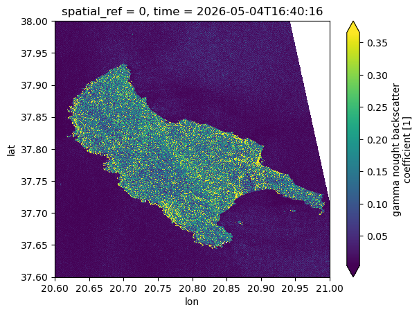
We now generate a data cube from the Sentinel-1 Level-1 GRD product by setting data_id to "sentinel-1-l1-grd". The bounding box is defined to cover Zakynthos, while the temporal range is restricted to a few days in May 2026.

We begin by creating the data cube in "EPSG:4326", which is the coordinate reference system (CRS) of the Copernicus DEM GLO-30 dataset used for geocoding and solving the inverse zero-Doppler equation.

bbox = [20.6, 37.6, 21.0, 38.0]
time_range = ["2026-05-04", "2026-05-05"]

%%time
ds = store.open_data(
    data_id="sentinel-1-l1-grd",
    bbox=bbox,
    time_range=time_range,
)
ds

CPU times: user 13.7 s, sys: 2.96 s, total: 16.7 s
Wall time: 42 s

Note: The calcuated indices during the inverse geodcoding process are written to a temporary directory. The remainder of the 3D data cube generation is lazy. Data access and processing operations (e.g., downloading, mosaicking, and stacking) are only executed on demand and are triggered when the data is explicitly computed, written, or visualized.

As an example, the following cell visualizes a single timestamp of the gamma nought VV backscatter band (gamma0_vv).

%%time
ds.gamma0_vv.isel(time=0).plot(robust=True)

/home/konstantin/micromamba/envs/eopf-zarr/lib/python3.11/site-packages/dask/_task_spec.py:768: RuntimeWarning: divide by zero encountered in divide
  return self.func(*new_argspec)

CPU times: user 2.33 s, sys: 475 ms, total: 2.8 s
Wall time: 3.33 s

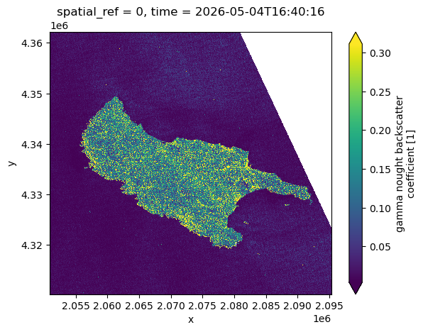
The same data cube can also be requested in a different coordinate reference system (CRS), such as UTM. The xcube-eopf framework supports on-the-fly reprojection to any user-defined CRS.

The resampling behavior can be customized when required. By default, bilinear interpolation is applied. Alternatively, nearest-neighbor interpolation can be selected, as shown below. See the xcube-resampling documentation for further details on available resampling and aggregation options.

Note: The requested spatial resolution and bounding box must be specified in the coordinate units of the target CRS.

crs_utm = "EPSG:32631"
bbox_utm = reproject_bbox(bbox, "EPSG:4326", crs_utm)

%%time
ds = store.open_data(
    data_id="sentinel-1-l1-grd",
    bbox=bbox_utm,
    time_range=time_range,
    spatial_res=30,  # in meter
    crs=crs_utm,
)
ds

CPU times: user 27.8 s, sys: 4.28 s, total: 32.1 s
Wall time: 45.6 s

And again, the following cell visualizes a single timestamp of the gamma nought VV backscatter band (gamma0_vv).

%%time
ds.gamma0_vv.isel(time=0).plot(robust=True)

CPU times: user 3.22 s, sys: 707 ms, total: 3.92 s
Wall time: 3.31 s

Access Sentinel-1 Level-1 SLC ARDC¶

In this section, we demonstrate the available features and options for opening and generating spatio-temporal data cubes from multiple Sentinel-1 Level-1 SLC tiles.

Note: Support for Sentinel-1 SLC products is currently experimental and under validation.

The opening parameters for this collection are shown below:

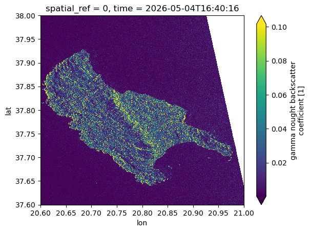
store.get_open_data_params_schema(data_id="sentinel-1-l1-slc")

Due to the computationally intensive processing, opening the data cube may take longer. In native mode, each TOPSAR burst is represented as a separate DataTree subgroup, resulting in a complex hierarchical structure that increases the time required to open and inspect the dataset. In analysis mode, additional processing steps such as debursting and burst merging are performed before further processing.

ds = store.open_data(
    data_id="sentinel-1-l1-slc",
    bbox=bbox,
    time_range=time_range,
)
ds

And again, the following cell visualizes a single timestamp of the gamma nought VV backscatter band (gamma0_vv).

%%time
ds.gamma0_vv.isel(time=0).plot(robust=True)

CPU times: user 4.37 s, sys: 892 ms, total: 5.26 s
Wall time: 14.3 s

Access Sentinel-1 Level-2 OCN ARDC¶

In this section, we demonstrate how to open and generate spatio-temporal data cubes from multiple Sentinel-1 Level-2 OCN observations.

The opening parameters for this collection are shown below:

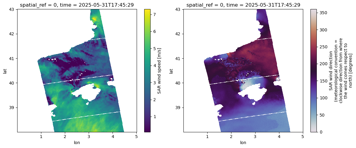
store.get_open_data_params_schema(data_id="sentinel-1-l2-ocn")

We set data_id to "sentinel-1-l2-ocn". As an example, we select the Balearic Islands and the surrounding Mediterranean Sea as the region of interest, with observations from the end of May 2025.

%%time
ds = store.open_data(
    data_id="sentinel-1-l2-ocn",
    bbox=[0, 38, 5, 43],
    time_range=["2025-05-27", "2025-05-31"],
)
ds

CPU times: user 3.67 s, sys: 152 ms, total: 3.82 s
Wall time: 12.9 s

The following cell visualizes the wind speed and wind direction side by side for a selected timestamp.

%%time
fig, ax = plt.subplots(1, 2, figsize=(12, 5))
ds.wind_speed.isel(time=-1).plot(ax=ax[0], cmap="viridis")
ds.wind_direction.isel(time=-1).plot(ax=ax[1], cmap="twilight", vmin=0, vmax=360)
plt.tight_layout()

CPU times: user 814 ms, sys: 65.3 ms, total: 880 ms
Wall time: 908 ms

Conclusion¶

This notebook highlighted the main features of the xcube EOPF Data Store for Sentinel-1, which enables seamless access to multiple EOPF Zarr products as analysis-ready data cubes (ARDCs).

Key takeaways:

3D spatio-temporal data cubes can be generated from multiple EOPF Sentinel Zarr samples.
Supports access to Sentinel-1 Level-1 GRD, Level-1 SLC, and Level-2 OCN collections.
Data cubes can be requested with any CRS, spatial extent, temporal range, and spatial resolution.