xarray EOPF backend - Sentinel-1 Analysis Mode

Table of Contents¶

Introduction
Main Features
Import modules
Open a Sentinel-1 Level-1 GRD
Open a Sentinel-1 Level-1 SLC
Open a Sentinel-1 Level-2 OCN
Conclusion

Run this notebook interactively with all dependencies pre-installed

Introduction¶

xarray-eopf is a Python package that extends xarray with a custom backend called "eopf-zarr". This backend enables seamless access to ESA EOPF data products stored in the Zarr format, presenting them as analysis-ready data structures.

In this notebook, we demonstrate how to use the xarray-eopf backend to access Sentinel-1 EOPF Zarr products in analysis mode. All data access is lazy, meaning that data is only loaded when required—for example, during plotting or when writing to storage.

For a general introduction to the xarray EOPF backend, see the introduction notebook. For an example of the native mode, see the Sentinel-1 native mode notebook.

🐙 GitHub: EOPF Sample Service – xarray-eopf
❗ Issue Tracker: Submit or view issues
📘 Documentation: xarray-eopf Docs

Main Features of the Analysis Mode for Sentinel-1¶

The Sentinel-1 analysis workflow supports:

Sentinel-1 GRD¶

Sentinel-1 GRD products are provided in radar geometry with the coordinates azimuth_time and ground_range. To generate an analysis-ready dataset, the following processing steps are performed:

Radiometric Calibration: Raw pixel values (DN) are converted to calibrated backscatter using the beta_nought calibration lookup table (LUT).
Geometric Terrain Correction (GTC): The data is geocoded by inverse geocoding using satellite orbit information and a Digital Elevation Model (DEM). This involves solving the zero-Doppler equation to map radar coordinates onto a georeferenced grid.
Radiometric Terrain Correction (RTC): Optionally compensates for terrain-induced radiometric effects such as foreshortening, layover, and slope-dependent brightness variations.

Reference

📖 D. Small, Flattening Gamma: Radiometric Terrain Correction for SAR Imagery

Sentinel-1 SLC¶

Sentinel-1 SLC products are provided as complex-valued bursts in radar geometry with the coordinates azimuth_time and slant_range_time. To generate an analysis-ready dataset, the following processing steps are performed:

Radiometric Calibration: Each burst is calibrated using the beta_nought calibration LUT. The complex-valued SLC data is converted to amplitude (abs(slc)).
TOPSAR Debursting: Individual bursts are aligned and merged into a continuous image. Burst overlaps are identified from the product metadata and removed.
Geometric Terrain Correction (GTC): Identical to the GRD workflow.
Radiometric Terrain Correction (RTC): Identical to the GRD workflow.

Sentinel-1 OCN¶

Sentinel-1 OCN products are provided on a geographic swath grid, where each pixel is defined by a latitude/longitude pair, forming a two-dimensional curvilinear (irregular) grid.

Analysis mode applies the xcube-resampling rectification algorithm to transform this irregular grid into a regular (rectilinear) grid with one-dimensional latitude and longitude coordinates.

Analysis Mode Features¶

The following features are available for all Sentinel-1 product types:

Default operation mode for the "eopf-zarr" backend
Lazy processing using Dask
Flexible variable selection using explicit variable names or regular expressions
Configurable interpolation via interp_methods (nearest, bilinear)

Features specific to GRD and SLC¶

Flexible output grid definition
- Supply a DEM directly via the dem parameter (xarray.DataArray).
- Or define the target grid using crs, bbox, and resolution.
- If no DEM is supplied, the CopDEM COG (30 m) is retrieved automatically via the CDSE STAC API (requires CDSE S3 credentials).
Optional Radiometric Terrain Correction (RTC) via apply_rtc=False.
Configurable radar footprint scaling through footprint_scale_factor, which controls how radar pixels contribute to the output grid.
- GRD default: (3.0, 3.0) to account for the resolution difference (e.g. ~10 m GRD vs. ~30 m DEM).
- SLC default: (3.0, 15.0) to account for the resolution difference (e.g. ~10 m × ~2 m SLC vs. ~30 m DEM).

Features specific to OCN¶

Rectification from a 2D curvilinear grid to a rectilinear grid
Spatial subsetting via bbox
Reprojection to arbitrary CRSs via crs (default: WGS84 / EPSG:4326)

For a complete description of the available opening parameters, see the Analysis Mode documentation and the Sentinel-1 Analysis Mode guide.

Import Modules¶

The eopf-zarr backend is registered as an xarray plugin. Import xarray as usual, plus helper libraries used in this notebook.

import os
import datetime

import matplotlib.pyplot as plt
import pystac_client
import xarray as xr
from xcube_resampling.utils import reproject_bbox

Open a Sentinel-1 Level-1 GRD Product in Analysis Mode¶

We begin with an example that accesses a Sentinel-1 Level-1 GRD product in analysis mode.

Find a Sentinel-1 GRD Zarr Sample via STAC¶

To obtain a product URL, you can use the STAC Browser to search for a Sentinel-1 GRD tile.

%%time
bbox = [20.6, 37.6, 21.0, 38.0]
catalog = pystac_client.Client.open("https://stac.core.eopf.eodc.eu")
items = list(
    catalog.search(
        collections=["sentinel-1-l1-grd"],
        bbox=bbox,
        datetime=[str(datetime.date.today() - datetime.timedelta(days=30)), None],
    ).items()
)
items

CPU times: user 31 ms, sys: 2 ms, total: 33 ms
Wall time: 1.62 s

[<Item id=S1D_IW_GRDH_1SDV_20260717T163121_20260717T163146_003716_006A72_8B2D>,
 <Item id=S1C_IW_GRDH_1SDV_20260717T043906_20260717T043931_008578_010FD0_A583>,
 <Item id=S1C_IW_GRDH_1SDV_20260716T163859_20260716T163924_008571_010F8C_7D8E>,
 <Item id=S1C_IW_GRDH_1SDV_20260711T163057_20260711T163122_008498_010D2F_A73D>,
 <Item id=S1D_IW_GRDH_1SDV_20260711T043919_20260711T043944_003621_006736_C9AC>,
 <Item id=S1D_IW_GRDH_1SDV_20260710T163924_20260710T163949_003614_006700_B3C3>,
 <Item id=S1D_IW_GRDH_1SDV_20260710T163859_20260710T163924_003614_006700_1481>,
 <Item id=S1D_IW_GRDH_1SDV_20260705T163120_20260705T163145_003541_006487_5456>,
 <Item id=S1D_IW_GRDH_1SDV_20260705T163055_20260705T163120_003541_006487_45CD>,
 <Item id=S1C_IW_GRDH_1SDV_20260705T043906_20260705T043931_008403_010A0D_E6E0>,
 <Item id=S1C_IW_GRDH_1SDV_20260704T163858_20260704T163923_008396_0109D0_A02C>,
 <Item id=S1C_IW_GRDH_1SDV_20260629T163056_20260629T163121_008323_01077A_7C35>,
 <Item id=S1D_IW_GRDH_1SDV_20260629T043918_20260629T043943_003446_006150_2CFD>,
 <Item id=S1D_IW_GRDH_1SDV_20260628T163924_20260628T163949_003439_006113_06DF>,
 <Item id=S1D_IW_GRDH_1SDV_20260628T163859_20260628T163924_003439_006113_77AD>,
 <Item id=S1A_IW_GRDH_1SDV_20260628T163159_20260628T163224_065172_08372A_992E>,
 <Item id=S1A_IW_GRDH_1SDV_20260628T163134_20260628T163159_065172_08372A_C838>,
 <Item id=S1D_IW_GRDH_1SDV_20260623T163109_20260623T163134_003366_005EA4_1276>,
 <Item id=S1A_IW_GRDH_1SDV_20260622T044013_20260622T044038_065077_0833E1_8D63>]

item = items[1]
item

Open Sentinel-1 GRD with default parameters¶

We can now open the Sentinel-1 product in analysis mode. Since this is the default, the op_mode parameter does not need to be specified.

The following cell returns a lazy dataset. For demonstration purposes, we restrict the data to a small spatial subset by specifying a bounding box.

Before proceeding, CDSE S3 credentials must be configured to enable access to the CopDEM (30 m) dataset from CDSE. Instructions for generating credentials are available here.

os.environ.update(
    {
        "AWS_ACCESS_KEY_ID": "xxx",
        "AWS_SECRET_ACCESS_KEY": "xxx",
    }
)

%%time
ds = xr.open_dataset(
    item.assets["product"].href, engine="eopf-zarr", bbox=bbox, chunks={}
)
ds

CPU times: user 5.25 s, sys: 1.32 s, total: 6.57 s
Wall time: 24.3 s

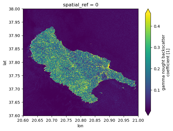
As an example, we plot the calibrated VV polarization band. Plotting triggers lazy loading and computation.

%%time
ds.gamma0_vv.plot(robust=True)

/home/konstantin/micromamba/envs/eopf-zarr/lib/python3.11/site-packages/dask/_task_spec.py:768: RuntimeWarning: divide by zero encountered in divide
  return self.func(*new_argspec)

CPU times: user 2.47 s, sys: 518 ms, total: 2.99 s
Wall time: 4.18 s

Open Sentinel-1 GRD in UTM grid¶

In the following we show different ways to open a Sentinel-1 GRD product in analysis mode.

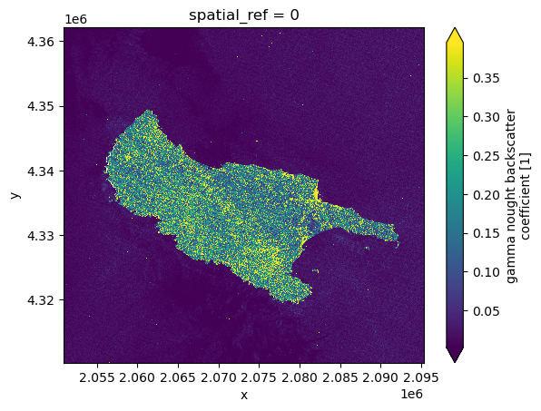
We can define the target gridmapping in UTM using the resolution, crs,and bbox parameters.

%%time
crs_utm = "EPSG:32631"
bbox_utm = reproject_bbox(bbox, "EPSG:4326", "EPSG:32631")

ds = xr.open_dataset(
    item.assets["product"].href,
    engine="eopf-zarr",
    bbox=bbox_utm,
    crs=crs_utm,
    resolution=30,  # meters
    chunks={},
)
ds

CPU times: user 7.59 s, sys: 1.5 s, total: 9.09 s
Wall time: 20.5 s

We can again visualize one polarization channel (for example vv).

%%time
ds.gamma0_vv.plot(robust=True)

CPU times: user 2.78 s, sys: 637 ms, total: 3.42 s
Wall time: 4.01 s

Turn off radiometric terrain correction (RTC)¶

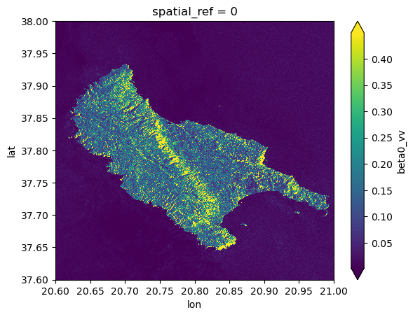
In the next example we turn off the RTC and select on the vv band.

%%time
ds = xr.open_dataset(
    item.assets["product"].href,
    engine="eopf-zarr",
    bbox=bbox,
    variables=["vv"],
    apply_rtc=False,
    chunks={},
)
ds

CPU times: user 3.19 s, sys: 521 ms, total: 3.71 s
Wall time: 11.3 s

In the following plot you can clearly see the structure of the mountainous terrain, since the backscatter variation has not been corrected for the terrain.

%%time
ds.beta0_vv.plot(robust=True)

CPU times: user 1.11 s, sys: 267 ms, total: 1.37 s
Wall time: 3.95 s

Interpolation Method: Nearest Neighbor¶

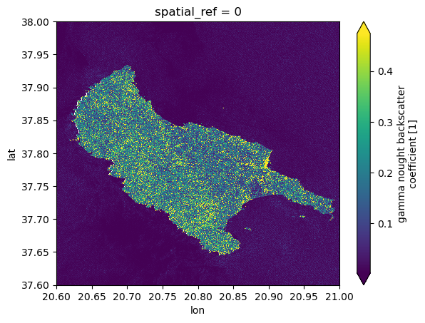
In the next example, we set the interpolation method to nearest, which is applied during both Geometric Terrain Correction (GTC) and Radiometric Terrain Correction (RTC).

This approach improves computational performance but reduces accuracy compared to bilinear interpolation, as it avoids spatial smoothing and instead assigns the value of the closest pixel.

%%time
ds = xr.open_dataset(
    item.assets["product"].href,
    engine="eopf-zarr",
    bbox=bbox,
    interp_methods="nearest",
    chunks={},
)
ds

CPU times: user 3.74 s, sys: 796 ms, total: 4.54 s
Wall time: 13.8 s

%%time
ds.gamma0_vv.plot(robust=True)

CPU times: user 1.36 s, sys: 316 ms, total: 1.68 s
Wall time: 4.06 s

Open a Sentinel-1 Level-1 SLC Product in Analysis Mode¶

Next, we show an example that accesses a Sentinel-1 Level-2 SLC product in analysis mode.

Find a Sentinel-1 SLC Zarr Sample via STAC¶

To obtain a product URL, you can use the STAC Browser to search for a Sentinel-1 SLC tile.

%%time
bbox = [20.6, 37.6, 21.0, 38.0]
catalog = pystac_client.Client.open("https://stac.core.eopf.eodc.eu")
items = list(
    catalog.search(
        collections=["sentinel-1-l1-slc"],
        bbox=bbox,
        datetime=["2026-05-04", "2026-05-04"],
        # datetime=[str(datetime.date.today() - datetime.timedelta(days=180)), None],
    ).items()
)
items

CPU times: user 24.1 ms, sys: 2.49 ms, total: 26.6 ms
Wall time: 222 ms

[<Item id=S1A_IW_SLC__1SDV_20260504T164002_20260504T164029_064370_081B0C_287A>]

item = items[0]
item

%%time
ds = xr.open_dataset(
    item.assets["product"].href, engine="eopf-zarr", bbox=bbox, chunks={}
)
ds

CPU times: user 12.4 s, sys: 1.05 s, total: 13.4 s
Wall time: 1min 28s

As an example, we plot the calibrated VV polarization band. Plotting triggers lazy loading and computation.

%%time
ds.gamma0_vv.plot(robust=True)

CPU times: user 4.8 s, sys: 856 ms, total: 5.65 s
Wall time: 13.4 s

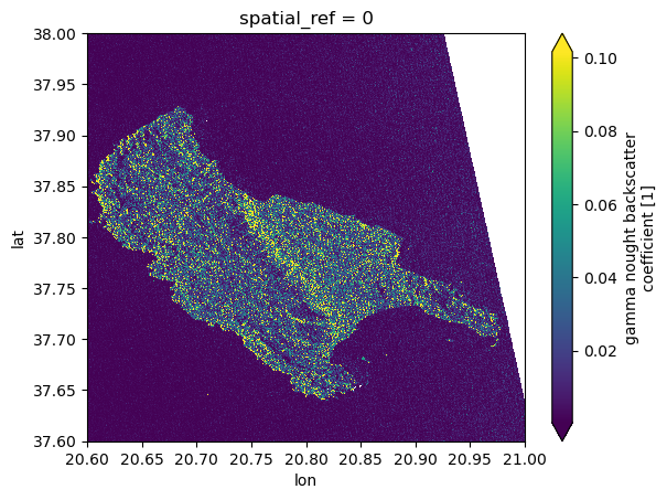
The same functionalities available for GRD products are also supported for SLC products, including the selection of different CRSs, bounding boxes, spatial resolutions, and interpolation methods.

Open a Sentinel-1 Level-2 OCN Product in Analysis Mode¶

Next, we show an example that accesses a Sentinel-1 Level-2 OCN product in analysis mode.

Find a Sentinel-1 OCN Zarr Sample via STAC¶

To obtain a product URL, you can use the STAC Browser to search for a Sentinel-1 OCN tile.

%%time
bbox = [3.0, 39.4, 3.2, 39.6]
catalog = pystac_client.Client.open("https://stac.core.eopf.eodc.eu")
items = list(
    catalog.search(
        collections=["sentinel-1-l2-ocn"],
        bbox=bbox,
        datetime=[str(datetime.date.today() - datetime.timedelta(days=365)), None],
    ).items()
)
items

CPU times: user 23.7 ms, sys: 2.5 ms, total: 26.2 ms
Wall time: 208 ms

[<Item id=S1A_IW_OCN__2SDV_20250730T055348_20250730T055413_060309_077EBE_1CA3>]

item = items[0]

%%time
ds = xr.open_dataset(
    item.assets["product"].href,
    engine="eopf-zarr",
    chunks={},
)
ds

CPU times: user 167 ms, sys: 4.03 ms, total: 171 ms
Wall time: 951 ms

%%time
fig, ax = plt.subplots(1, 2, figsize=(12, 5))
ds.wind_speed.plot(ax=ax[0], cmap="viridis")
ds.wind_direction.plot(ax=ax[1], cmap="twilight", vmin=0, vmax=360)
plt.tight_layout()

CPU times: user 270 ms, sys: 18.3 ms, total: 288 ms
Wall time: 477 ms

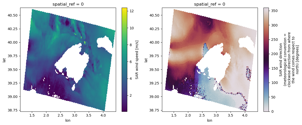
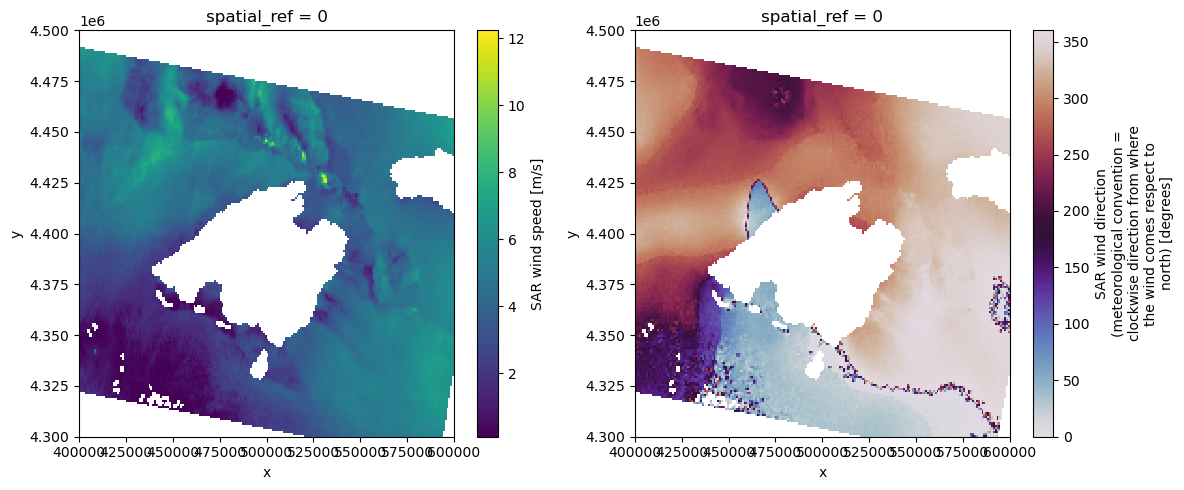
We can also request the data in a different CRS, and define the target grid mapping by using the parameters resolution, and bbox.

%%time
ds = xr.open_dataset(
    item.assets["product"].href,
    engine="eopf-zarr",
    crs="EPSG:32631",
    resolution=1_000,  # meters
    bbox=[4e5, 4.3e6, 6e5, 4.5e6],
    variables=["wind_direction", "wind_speed"],
    chunks={},
)
ds

CPU times: user 297 ms, sys: 12.5 ms, total: 309 ms
Wall time: 1.19 s

%%time
fig, ax = plt.subplots(1, 2, figsize=(12, 5))
ds.wind_speed.plot(ax=ax[0], cmap="viridis")
ds.wind_direction.plot(ax=ax[1], cmap="twilight", vmin=0, vmax=360)
plt.tight_layout()

CPU times: user 169 ms, sys: 22.8 ms, total: 192 ms
Wall time: 253 ms

Conclusion¶

This notebook demonstrates how to access Sentinel-1 EOPF Zarr samples in analysis mode using the xarray-eopf plugin.

The main characteristics of analysis mode are:

Analysis mode is the default op_mode and therefore does not need to be specified explicitly.
Data is accessed lazily and processed on demand for a user-defined CRS, bounding box, and spatial resolution, enabling efficient subsetting, reprojection, and resampling.

Sentinel-1 Level-1 GRD¶

The analysis workflow for Sentinel-1 Level-1 GRD includes:

Radiometric calibration using the product LUTs.
Geometric Terrain Correction (GTC) through inverse geocoding using orbit information and a DEM.
Optional Radiometric Terrain Correction (RTC) to compensate for terrain-induced radiometric distortions.
A DEM can either:
- be provided explicitly by the user, or
- be retrieved automatically from the CDSE STAC API and resampled to user-defined CRS, bounding box, and spatial resolution.
If a DEM is provided, its grid definition determines the output grid.

Sentinel-1 Level-1 SLC¶

The analysis workflow for Sentinel-1 Level-1 SLC includes:

Radiometric calibration of each burst using the product LUTs.
TOPSAR debursting, in which individual bursts are merged into a continuous image.
Geometric Terrain Correction (GTC) through inverse geocoding using orbit information and a DEM.
Optional Radiometric Terrain Correction (RTC) to compensate for terrain-induced radiometric distortions.
A DEM can either:
- be provided explicitly by the user, or
- be retrieved automatically from the CDSE STAC API and resampled to user-defined CRS, bounding box, and spatial resolution.
If a DEM is provided, its grid definition determines the output grid.
Apart from the additional TOPSAR debursting step, the same configuration options as for GRD are available.

Sentinel-1 Level-2 OCN¶

The analysis workflow for Sentinel-1 Level-2 OCN includes:

Rectification from the native irregular latitude/longitude swath grid to a regular target grid.
User-defined output grids via the crs, bbox, and resolution parameters.
Automatic inclusion of quality flag variables by default.
Optional variable selection using the variables parameter.

Note: This notebook focuses exclusively on analysis mode. To learn more about native mode, see the Sentinel-1 native mode notebook.